


 Inglés (pdf)
 Articulo en XML
 Referencias del artículo
 Enviar articulo por email
 Citado por SciELO
  Similares en
SciELO
Similares en
SciELO 
 Permalink
INTRODUCTION
The root system is responsible for the uptake of soil water and nutrients, and plant physical support (Taiz et al., 2017). Dry mass, surface area, and length are commonly measured to assess or model the efficiency of water and nutrient uptake by roots (Nye and Tinker, 1977); most measurements focus on the fine roots (diameter ≤2 mm) because of their high relevance in the uptake process (Schroth, 1999). However, the measurement of such root variables is extremely laborious and time-consuming (Böhm, 1979), and thus, there is a great need for research methods that minimize the effort and time spent in root studies.
Data on specific root length and surface area are very limited due to insufficiency of studies involving root length measurement. Related methods such as the line-intersect (Newman, 1966; Marsh, 1971; Tennant, 1979) and direct measurement (Ahlrichs et al., 1990) are considered as standards for assessing root length, but they are laborious and time-consuming (Tennant, 1979) and present low accuracy because of human subjectivity (Judd et al., 2015). The error in a direct measurement and line-intersect methods can range from 2 to 5% (Newman, 1966).
Automatic and semi-automatic methods that are based on the analysis of root images are more efficient than non-automatic (line-intersect and direct measurement) methods for estimating root length, area, and diameter (Vamerali et al., 2003; Delory et al., 2017). Image analysis softwares are used in automatic and semi-automatic methods, such as the Safira software, developed by the Brazilian Agricultural Research Corporation (Embrapa), and the ImageJ software, developed by the National Institute of Health (NIH), USA. The few studies that assessed the accuracy of both Safira and ImageJ (Tanaka et al., 1995; Costa et al., 2014; Delory et al., 2017) have focused on the fine roots of short-cycle crops, probably due to their agronomic relevance. Fewer related studies have focused on the coarse roots (diameter >2 mm) despite their significant contribution to the whole root system biomass and belowground carbon pool. In oil palm (Elaeis guineensis Jacq.), for example, coarse roots represent approximately 84% of the total root biomass (Gloria, 2016). Oil palm is a commodity of African origin whose oil extracted from its fruits represents the main raw material of the oilseed industry in the world (Corley & Tinker, 2016). It accounts for 38.8% of all vegetable oil sold in the world, with a total of 70 million tons (between 2017 and 2018); Brazil supplies 0.72% of this amount (USDA, 2018).
The root architecture (Jourdan & Rey, 1996, 1997a, b) and biomass (Rees & Tinker, 1963; Corley et al., 1971; Cuesta et al., 1997; Jourdan et al., 2000; Kiyono et al., 2015; Sanquetta et al., 2015) of oil palm have been relatively well studied. However, few studies have distinguished between root diameter classes (Corley & Tinker, 2016), and there is a still lack of estimates of oil palm root length (Yahya et al., 2010). Thus, it is necessary to develop simple, accurate protocols to estimate the root length of the different root classes of oil palm. Here we assessed the accuracy of different methods to estimate them.
MATERIALS AND METHODS
We conducted this study at the Laboratory of Sustainable Systems Analysis (LASS) of Embrapa Amazônia Oriental, Pará, Brazil, between August and October 2017. We used segments of oil palm roots, as well as electric and nylon wires of known diameters, to evaluate the accuracy of methods to estimate oil palm root length - one non-automatic method (line-intersect, Tennant) and two methods based on image analysis software (Safira and ImageJ).
We collected roots of an interspecific oil palm hybrid (Elaeis guineensis Jacq. x Elaeis oleifera (Kunth) Cortés) from a 10-yr-old commercial plantation (Marborges S/A) in the municipality of Moju, Pará, Brazil. The plants were arranged in an equilateral triangle with 9x9 m spacing. We collected one soil monolith (approximate dimensions: width = 0.5 m, length = 0.4 m, depth = 0.3 m) 1 m away from two individuals. We washed the soil samples in running water and stored the roots under refrigeration (~5 °C) for 24 h. Then we separated the roots according to diameter class into primary (5-10 mm), secondary (1-4.9 mm), tertiary (0.5-0.9 mm), and quaternary (0.2-0.49 mm) (adapted from Corley & Tinker, 2016).
After classification, we randomly selected 15 root segments (root segment pool) of each diameter class and cut the primary, secondary, and tertiary roots into sections of approximately 10 cm in length. Due to the absence of quaternary roots with length ≥10 cm, we picked the 15 longest sections (mean of 3.3 cm) of this root class. For each diameter class, we formed ten samples composed of five root segments each - randomly selected among the 15 root segments, with the replacement of segments to the root segment pool after measuring each sample (described below). Then we randomly selected the next sample and so on (sampling with replacement approach).
To determine the percent error variation of the root length estimates of Tennant, Safira, and ImageJ methods in relation to the reference one (direct measurement), we used wires with diameters of 6.9, 2.75, 0.75, and 0.35 mm which were respectively close to the intermediate value of the diameter range of the primary, secondary, tertiary, and quaternary roots. We used electric wires for the larger diameters (2.75 and 6.9 mm), and nylon wires for the other widths. We painted the wires with black automotive paint to standardize the color and enhance image contrast for scanning. Then we cut the wires into segments of approximately 10 cm in length. In the direct measurement (DM) method, considered as reference in this study, we measured the length of each wire or root segment to the nearest millimeter with a ruler.
In the line-intersect method (Tennant, 1975), we randomly arranged the samples (without root overlapping) on an A4 size paper sheet. We used 2x2 cm squared paper sheets for the primary roots and 6.9 mm diameter wires, and 1x1 cm sheets for the other diameter classes of roots and wires. We applied the equation L=1.5714 x N x G for the primary roots and 6.9 mm diameter wires and the equation 𝐿=0.7857 x N x G for the other diameter classes of roots and wires. For both equations, L is the total length, N is the number of intersects, and G is the grid unit (Tennant, 1975). We registered the time demanded to obtain the total length of each sample.
In the image analysis methods, we scanned the root and wire samples using a flatbed scanner (Canon, Pixma MP280) with 319 x 418 DPI resolution. Before scanning, we placed a 10 cm millimeter ruler next to each sample to calibrate the scale in the software further. We converted each scanned image into a binary image. The average time spent for image acquisition and conversion into the binary was 1.3 min, which was added to the average time of analyses of each software. We analyzed the images using Safira V.1.1 (Jorge & Silva, 2010), developed by Embrapa, and the plugin Smartoot of ImageJ V.1.46 (ImageJ, 1997), developed by the National Institute of Health, USA (Figure 1).
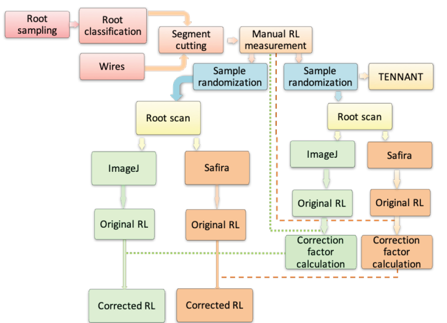
For the ImageJ software, we used the pixel/cm information (obtained with the software calibration option and the ruler reference in the image) for calibration because this procedure resulted in higher accuracy compared to using a fixed, default resolution value. We used the following values: 31,500 pixels/cm for the primary, secondary, and tertiary roots; 23,802 pixels/cm for the quaternary roots; 23,601 pixels/cm for the 6.9 and 2.5 mm wires; 158,16 pixels/cm for the 0.7 mm wire; and 156,91 pixels/cm for the 0.35 mm wire. We noticed that the automatic drawing mode underestimated root length since parts of the segments of the tertiary and quaternary roots were not recognized as roots. For these root diameter classes, we used the Traceroot tool, which did not underestimate root length. We initially calibrated the Safira software using the reference scale (ruler) in each image. Then we adjusted the thresholds before running the analysis.
We applied the root estimates from both the Safira and ImageJ analyses to obtain correction factors (CF) of each root class, based on the following equation:
CF = ( 𝐿𝑅−𝐿𝐸 𝐿𝑅 ),
where LR is the real root length (determined by the manual method), and LE is the length estimated by the software. We then applied the equation
LC = LE + LE(( CF
to correct the root length, where LC is the corrected length. We then randomly selected another set of oil palm root segments (10 samples with five individual root images per sample) for image analysis using both Safira and ImageJ; we applied the correction factors to these estimates.
We applied the Paired sample t-test, with n=10 at 5% significance level, to compare each method individually (Tennant, Safira, ImageJ) against the reference (direct method). We used nonparametric statistics to analyze the corrected length of secondary and quaternary roots. We used the SigmaPlot 12.0 software for all statistical analysis.
RESULTS AND DISCUSSION
In general, the image analysis softwares (Safira and ImageJ) and the Tennant method showed limited accuracy to estimate root length. For some root diameter classes, estimates of these methods differed significantly from the results of the reference method. Root length values estimated by the Safira software differed significantly from the values determined by the reference method for all root classes (Table 1). The average time spent to measure each root class ranged from 2 to 4 min using the Safira software. The ImageJ software was accurate to estimate the length of quaternary roots, but for the other root classes (primary, secondary, and tertiary), the estimates differed significantly from the results of the reference method. The time for analysis of each root class was approximately 5.3 to 10 min using the ImageJ software. The Tennant method did not differ from the reference method to estimate the length of tertiary and quaternary roots; the average analysis time varied between 1.00 and 1.20 min.
Table 1 Length of primary, secondary, tertiary, and quaternary oil palm roots determined manually (reference) and estimated by the line-intersect method (Tennant) and image analysis methods (Safira and ImageJ). Time refers to the total duration of processing and analysing the root samples
| Primary root | Secondary root | Tertiary root | Quaternary root | ||||||||||
| Method | Length (cm)1 | Time (min) | Length (cm) | Time (min) | Length (cm) | Time (min) | Length (cm) | Time (min) | |||||
| Reference | 51.06 ± 0.10 | 00:23.56 | 50.66 ± 0.04 | 00:29.07 | 50.59 ± 0.09 | 00:36.35 | 16.62 ± 0.21 | 00:55.60 | |||||
| Tennant | 54.37 ± 1.20* | 01:21.28 | 46.83 ± 0.43* | 01:21.27 | 50.13 ± 0.59 | 01:24.39 | 16.66 ± 0.52 | 01:12.83 | |||||
| Safira | 53.65 ± 0.49* | 02:16.45 | 52.02 ± 0.19* | 02:38.82 | 53.24 ± 0.20* | 02:51.78 | 17.02 ± 0.17* | 03:36.47 | |||||
| ImageJ | 50.84 ± 0.16* | 05:31.29 | 50.10 ± 0.06* | 05:56.77 | 50.88 ± 0.12* | 10:03.89 | 16.54 ± 0.20 | 07:52.47 | |||||
1Length data are mean ± standard deviation (n=10).
Asterisks indicate significant difference between a method and the reference according to the Paired sample t-test at 5% significance level.
Few studies have analyzed the time spent for root analysis using the line-intersect method; we are not aware of related studies using Safira. The use of automatic drawing in ImageJ reduces root analysis time compared to other methods (Kimura et al., 1999; Delory et al., 2017). However, the accuracy of root estimates with the ImageJ software may be strongly affected by the automatic drawing resource, leading to relative root length errors of 7% (Tanaka et al., 1995). Thus, such trade-offs between automatic drawing (which is less time-consuming) and accuracy should be accounted for before selecting a root analysis protocol.
The accuracy of each method was also assessed based on estimates using wires. The estimate of the length of 0.35 mm wires using the Tennant method and the ImageJ software did not differ from the value estimated by the reference method (Table 2); however, the ImageJ underestimated length in 0.24% and the Tennant overestimated it in 0.66%. These results are consistent with another study that tested 0.3 mm diameter wires using ImageJ (Kimura et al., 1999). Length estimates for the 6.9 mm diameter wires did not differ between the Safira software and the direct method (Table 2). For the intermediate diameters (0.75 and 2.5 mm), the non-direct methods (Tennant, Safira, ImageJ) differed from the directed method (Table 2). However, the ImageJ software showed the lowest relative difference to the direct measurement for all root classes.
Table 2 Wire length determined manually (reference) and estimated by the line-intersect method (Tennant) and image analysis methods (Safira and ImageJ). Error refers to the relative difference of each wire length value relative to the reference
| 6.95 mm-wire | 2.5 mm-wire | 0.75 mm-wire | 0.35 mm-wire | ||||||||
| Method | Length (cm)1 | Error (%) | Length (cm) | Error (%) | Length (cm) | Error (%) | Length (cm) | Error (%) | |||
| Reference | 50.2±0.05 | - | 50.00±0.00 | - | 50.00±0.00 | - | 50.11±0.02 | - | |||
| Tennant | 53.58±1.25* | 6.7 | 51.54±0.65* | 3.1 | 51.78±0.43* | 3.6 | 50.44±0.49 | 0.7 | |||
| Safira | 50.21±0.22 | 0 | 53.56±0.50* | 6.6 | 51.46±1.05* | 2.4 | 52.32±0.20* | 4.2 | |||
| ImageJ | 49.40±0.13* | -1.6 | 50.20±0.02* | 0.4 | 49.70±0.02* | -0.6 | 49.99±0.09 | -0.2 |
1Length data are mean ± standard deviation (n=10).
Asterisks identify results statistically different from the reference mean according to the Paired sample t-test at 5% significance level.
Percent error variation between analyses of wires and roots did not show a clear pattern (Table 3), that is, for a given root diameter class and its respective wire pattern, there was both over- and under-estimation depending on the root length measuring method, as reported by Delory et al. (2017). In the Tennant method, the larger diameter range of the secondary roots (1.0-4.9 mm) may have caused the high relative error of root length, considering that such error did not occur with the respective wire standard (2.5 mm diameter).The Tennant method is subject to sources of errors that image analysis softwares does not present, such as the involuntary omission of line intersects, error in intercept interpretation using Tennant guidelines, operator fatigue, and variation between operators (Delory et al., 2017). For example, operator variation may lead to a 10% error and different criteria of root arrangement may result in a 7% error (Bland & Mesarch, 1990).
Table 3 Relative error associated with the length of oil palm roots and wires estimated by the line-intersect method (Tennant) and image analysis softwares (Safira, ImageJ). Negative and positive signs indicate underestimation or overestimation, respectively
| Method | Primary root | 6.5 mm-wire | Secondary root | 2.5 mm- wire | Tertiary root | 0.75 mm-wire | Quaternary root | 0.35 mm-wire | |||
| Error (%) | Error (%) | Error (%) | Error (%) | ||||||||
| Tennant | 6.51 | 6.74 | -7.55 | 3.08 | -0.91 | 3.56 | 0.23 | 0.66 | |||
| Safira | 5.07 | 0.00 | 2.69 | 6.58 | 5.23 | 2.41 | 2.68 | 4.21 | |||
| ImageJ | -0.43 | -1.60 | -1.09 | 0.40 | 0.56 | -0.59 | -0.48 | -0.24 | |||
The correction factors did not entirely improve the accuracy of the Safira software (Table 4); the corrected length for primary (5-10 mm) and secondary (1-4.9 mm) roots differed statistically from those of the reference method. Thus, the use of correction factors to improve the accuracy of the Safira software is useful only when root diameters are in the range of 0.35-0.99 mm.
Table 4 Length of primary, secondary, tertiary, and quaternary oil palm roots determined by the reference method and estimated by image analysis softwares (Safira, ImageJ). Original and corrected length estimates are shown for both Safira and ImageJ
| Reference | Safira | ImageJ | |||||||||
| Root | Length (cm)1 | Original length (cm) | Corrected length (cm) | p | % | Original length (cm) | Corrected length (cm) | p | % | ||
| Primary | 51.13 ± 0.08 | 52.98 ± 0.36* | 50.30 ± 0.34* | 0.06 | 1.54 | 50.91 ± 0.07 | 51.13 ± 0.07 | 0.84 | -0.03 | ||
| Secondary | 50.56 ± 0.05 | 54.43 ± 0.52* | 52.97 ± 0.51* | 0.08 | 4.37 | 50.37 ± 0.04* | 50.81 ± 0.12 | <0.05 | 0.49 | ||
| Tertiary | 50.63 ± 0.05 | 54.02 ± 0.17* | 51.20 ± 0.16 | 0.01 | 1.13 | 51.08 ± 0.18* | 50.79 ± 0.18 | 0.40 | 0.33 | ||
| Quaternary | 16.54 ± 0.23 | 16.68 ± 0.19* | 16.24 ± 0.18 | 0.11 | 1.81 | 16.34 ± 0.24 | 16.40 ± 0.24 | 0.56 | 0.80 |
1Length data are mean ± standard deviation (n=10).
Asterisks indicate significant difference between means of an image analysis method and the reference according to the Paired sample t-test at 5% significance level.
ImageJ usually underestimates root length (Tanaka et al., 1995). Our results showed underestimation of primary (0.43%), secondary (1.09%), and quaternary roots (0.38%), although tertiary root length was overestimated by 0.56%. Such variation led to reduced accuracy of uncorrected estimates of some root diameter classes (Table 4). After applying the correction factor (Table 5), none of the estimates using the ImageJ software differed from the values of the reference method (Table 4).
Table 5 Correction factor for estimating oil palm root length using the ImageJ software. Negative and positive signs indicate underestimation or overestimation, respectively
| Primary root | Secondary root | Tertiary root | Quaternary root | |||
| Correction factor (%L) | ||||||
| -0.43 | -1.09 | 0.56 | -0.38 | |||
Despite the adequate accuracy of the ImageJ software, this tool showed the longest image analysis processing time in relation to the other methods, including the direct measurement (Table 1). However, in our study, we did not account for the time spent to separate the roots into different diameter classes. Such procedure is not necessarily required for the image analysis method using the ImageJ software, which may automatically classify the root segments into different root diameter intervals. In the direct measurement, a prior separation of roots in diameter classes (primary, secondary, etc.) is necessary to reduce the variance in the length estimate due to root overlapping (Tennant, 1988). Thus, the time spent in the reference method was underestimated in this study.

