


 Inglês (pdf)
 Artigo em XML
 Referências do artigo
 Enviar este artigo por email
 Citado por SciELO
  Similares em
SciELO
Similares em
SciELO 
 Permalink
Introduction
Both the concepts of potential evapotranspiration (PET) and reference evapotranspiration (ETo) (in increasing use) refer to reference surfaces with non-limiting water (Allen et al., 1998). They are only influenced by the action of climatic elements, thus becoming climatic parameters computable from meteorological or climate data. They have numerous applications, eg., in Agronomy, Climatology, Agrometeorology or Hydrology, and serve as a basis for assessing crop water requirements (Penman, 1948) leading to significant improvements in agricultural water use (Hargreaves & Samani, 1985), especially when land productivity is severely limited by water availability or supply (Doorembos & Pruitt, 1977). As its assessment allows for predicting the final crop yield, ETo is frequently used in various crop growth models (Pereira et al., 2015). As a component of the soil water balance, its evaluation for different time scales (daily, monthly...) is essential for calculating the variation in soil water storage (Thornthwaite, 1948), being crucial for scheduling irrigation (Jensen & Allen, 2016; Sharma, 1985) and enhancing water use efficiency. In different climate classifications, both concepts are used as a central parameter (e.g., Thornthwaite's Rational Classification of Climate, Köppen classification). Both indicators are also key components used in many analyses and mapping applications (e.g. GIS mapping software).
Many methods have been proposed (and used) to estimate ETo. They differ from each other not only by the number of variables used (simplicity of computations), with direct implications for computational times, but also by their applicability to different climatic conditions. In addition to these factors, adaptability in overcoming missing data is also relevant for selecting the method that better assesses ETo in each case (Hargreaves & Allen, 2003). The Penman-Monteith (PM) method (Monteith, 1965; Penman, 1948) is considered a reference method by the Food and Agriculture Organization of the United Nations (FAO-UNESCO) (Allen et al., 1998) being and is therefore widely used to estimate ETo. It uses several climatic/meteorological parameters (temperature, air humidity, wind and radiation). However, the frequent unavailability of one or more of these parameters and/or the lack of reliable data often limit their use. For this reason, the use of other methods has been advised by the FAO itself, namely the Hargreaves-Samani (HS) method (Hargreaves & Samani, 1985), either to fill gaps in some stages of the implementation of the PM method or even to replace it when the available data is limited to temperature data.
Testing and calibrating the temperature-based HS equation against the PM method was the challenge proposed by Allen et al. (1998) that many authors accepted. In most of the studies carried out under very different climatic (or meteorological) conditions, regardless of the time scale considered, the ETo values obtained by these two methods were successfully correlated (relatively high correlation). Examples include many works carried out in a Mediterranean environment, whether in drier areas (Gavilán et al., 2006; Martinez-Cob & Tejero-Juste, 2004), in wetter areas (Paredes et al., 2018; Trajkovic, 2007) or including both (Itenfisu et al., 2000; Todorovic et al., 2013), and also in the semiarid and arid (Akhavan et al., 2019; Mohawesh & Talozi, 2012; Raziei & Pereira, 2013; Valipour & Eslamian, 2014), dry tropical (Silva et al., 2005), temperate/cold and humid (Syperreck et al., 2008; Xu & Singh, 2002). This means that although the HS method has been empirically developed based on data from arid to sub-humid locations, it seems to be able to successfully replace the PM method in a more generalized way. These high correlations, larger on a monthly scale than on a daily scale, allow calibrating the HS equation to minimize differences between the values obtained by both models. Since ETo(HS)/ETo(PM) is different from place to place (sometimes >1, sometimes <1), there is no single calibration factor. To avoid using a calibration factor for each location, many authors have tried to quantify the variation of the calibration factor depending on factors such as type of climate, proximity to the sea or wind speed. The results were not conclusive. For example, Allen et al. (1998), Temesgen et al. (1999) and, more recently Trajkovic (2007), found that high humidity conditions may result in an overestimation of ETo by HS. According to the study carried out by Todorovic et al. (2013) in 16 Mediterranean countries, the HS method tends to underestimate PM in more arid areas (and especially in windier ones) and overestimate it in more humid areas. This trend was also found at times of the year with lower ET (colder periods) (Droogers & Allen, 2002; Xu & Singh, 2002), whereas either in drier zones (Jensen & Allen, 2016; Temesgen et al., 2005) or in warmer periods (Droogers & Allen, 2002) ETo(PM) was underestimated. Tabari (2010), in a study carried out in Iran, found worse performance of the HS method (average daily values for a period of 19 years) in wetter and colder areas than in hotter and drier areas. On the contrary, Raziei and Pereira (2013) found lower quality fits for the same territory (Iran) in areas with greater aridity. Furthermore, Jabloun and Sahli (2008) obtained results that overestimate the ETo(PM) values in the interior of Tunisia and underestimate them in coastal locations.
The wind factor was also highlighted by several authors (Allen et al., 1998; Gavilán et al., 2006; Martinez-Cob & Tejero-Juste, 2004; Temesgen et al., 1999), as a relevant factor in explaining less successful fits between the results obtained by the two methods. This fact results mainly from the increased underestimation of the ETo by the HS method in the windiest locations, which would explain, according to Allen et al. (1998) and Temesgen et al. (2005), the results obtained by Todorovic et al. (2013) in the most arid areas of the Mediterranean. Thus, other factors (wind speed, in this case), more than the greater or lesser aridity of the climate, can be decisive in the calibration of the HS equation.
Another issue is how to calibrate the HS equation in order to minimize the differences between values obtained by the two methods, as measured by the root mean square error (RMSE). Many authors have calibrated the HS equation according to the most influential factors in its relationship with the reference method (e.g. proximity to the sea, altitude and, wind speed). Some calibrated the HS equation as a function of proximity to the sea (parameterized in most cases as relative humidity or temperature range). Hargreaves (1994) proposed different values for a calibration factor to be applied to the original formula ranging from 0.16 for the most inland areas to 0.19 for the coastal areas. This suggestion was later maintained by Allen et al. (1998), without, in any case, the degree of interiority having been duly quantified. Gavilán et al. (2006) obtained ETo values by the HS method that overestimated those obtained by the PM method in coastal zones, but with no visible trend when analysing the values found in inland zones.
The simplicity of the HS method (temperature as a driving element for ETo estimation) has given rise to a large number of proposals to improve its performance (e.g., Allen, 1993; Berti et al., 2014; Droogers & Allen, 2002; Jensen et al., 1997; Martinez-Cob & Tejero-Juste, 2004; Xu & Singh, 2002). Despite all attempts, many authors suggest a local calibration to solve the problem (e.g., Allen et al., 1998; Droogers & Allen, 2002; Rodrigues & Braga, 2021).
Largely due to its geographic location (Strahler & Strahler, 2005), almost the entire territory of Portugal has a Mediterranean-type climate (mild winter temperatures, and relatively hot and dry summers). According to the Köppen Climate Classification (Peel et al., 2007), this means Cs-type climates. In the north (more mountainous) and on the west coast predominates the Csb-variant (cool summer), whereas in the south and vast areas of the less mountainous or flat inland, the Csa-variant (warm summer) dominates. Residual patches of BS climates are found in the southeast of the mainland and on the island of Porto Santo (Madeira archipelago). Relatively abundant rainfall in the summer in some parts of the Azores archipelago justifies the presence of a Cf-type climate, without losing its Mediterranean facies. Proximity to the sea, altitude and, to a lesser extent, latitude/general circulation of the atmosphere (Ferreira, 2005) are the most active climatic factors. Despite the good correlations found between the ETo values obtained by the PM and the HS methods in regions with a similar climate (Mediterranean Basin), no work was found in the literature that fully assumes the climatic diversity of the Portuguese territory (climates Cs, BS, and Cf) as a conditioning factor for the use of the HS method as an alternative to PM. Only the Azores archipelago (Paredes et al., 2018) and part of southern Portugal (Rodrigues & Braga, 2021) were studied for this purpose. Furthermore, no analytical quantification was found of the influence (combined or not) of the climatic factors that seem to determine to a greater extent the calibration of the HS equation in regions with a Mediterranean climate (namely, proximity to the sea and wind speed).
The main objective of this article was to calibrate the HS equation so that it can replace the PM equation whenever justified. For this purpose, data from climatic elements recorded in locations spread across the entire territory of Portugal were used. Considering the influence of the factors that most affect the climate of the national territory (proximity to the sea and altitude), as well as the role of wind speed as a central factor in evapotranspiration, the suitability of the proposed calibration coefficients for regions with similar climates (Mediterranean context) were also discussed.
Methodology
Study area and data
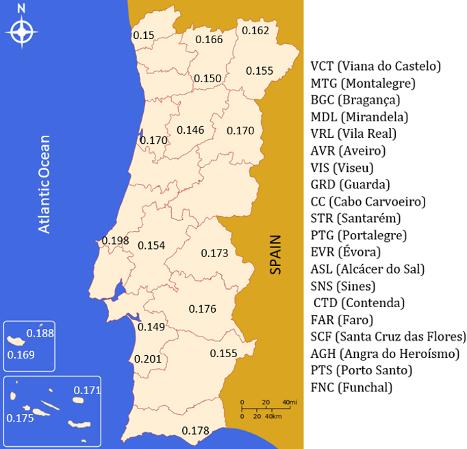
The study area comprises the entire Portuguese national territory (mainland and islands). Data from 20 weather stations belonging to the main meteorological network of the Portuguese Institute for Sea and Atmosphere (IPMA, IP) were used. Stations are identified by acronyms and corresponding names on figure 1. The choice of these locations reflected the country's existing climate diversity.
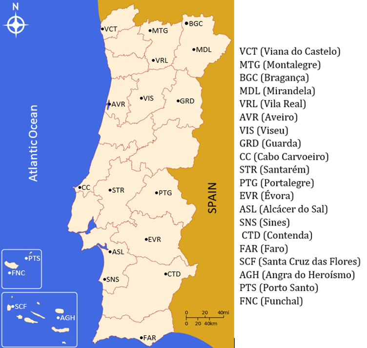
Table I shows the locations, geographic coordinates and distance to the sea of each weather station. Except for two stations located in the Madeira Archipelago (at around 32-33( North latitude), all are located between 37(01'N (FAR) and 41(49'N (MTG). According to the NUTS II classification (Level 2 of territorial units for statistical purposes) applied to the Portuguese territory, five stations are located to the North, five in the Centro, five in Alentejo, one in Algarve and two in each of the archipelagos (Azores and Madeira). Only GRD and MTG, both northern locations, are located above 1000 meters of altitude. BGC, VRL, VIS, PTG, and CTD are located between 400m and 700m altitude whereas all others are below 400 m. STR is the only non-coastal station located at an altitude of less than 100m. In the mainland, six out of 16 are coastal locations (VCT, AVR, CC, ASL, SNS, and FAR).
Table I Weather stations used: locations in Portuguese territory (NUTS II), coordinates (Latitude and longitude, in (), elevation (in meters) and distance from the sea (in kilometres).
| NUTS II | Weather Station | Latitude (North) | Longitude (West) | Elevation (m) | Distance to the Sea (Km) |
| Norte | MTG | 41(49’ | 7(47’ | 1005 | 89.5 |
| Norte | BGC | 41(48’ | 6(44’ | 690 | 175 |
| Norte | VCT | 41(42’ | 8(48’ | 16 | 1 |
| Norte | MDL | 41(31’ | 7(12’ | 250 | 132 |
| Norte | VRL | 41(19’ | 7(44’ | 481 | 83 |
| Centro | VIS | 40(40’ | 7(54’ | 443 | 70 |
| Centro | AVR | 40(38’ | 8(40’ | 5 | 8 |
| Centro | GRD | 40(32’ | 7(16’ | 1019 | 126 |
| Açores | SCF | 39(27’ | 31(07’ | 28 | 0.5 |
| Centro | CC | 39(21’ | 9(24’ | 32 | 0 |
| Alentejo | PTG | 39(17’ | 7(25’ | 597 | 166 |
| Centro | STR | 39(15’ | 8(42’ | 54 | 55 |
| Açores | AGH | 38(40’ | 27(13’ | 74 | 1 |
| Alentejo | EVR | 38(34’ | 7(54’ | 309 | 111 |
| Alentejo | ASL | 38(23’ | 8(31’ | 51 | 25 |
| Alentejo | CTD | 38(03’ | 7(04’ | 450 | 155 |
| Alentejo | SNS | 37(57’ | 8(53’ | 15 | 0 |
| Algarve | FAR | 37(01’ | 7(58’ | 8 | 4 |
| Madeira | PTS | 33(04' | 16(20' | 78 | 2 |
| Madeira | FNC | 32(38’ | 16(53’ | 58 | 0 |
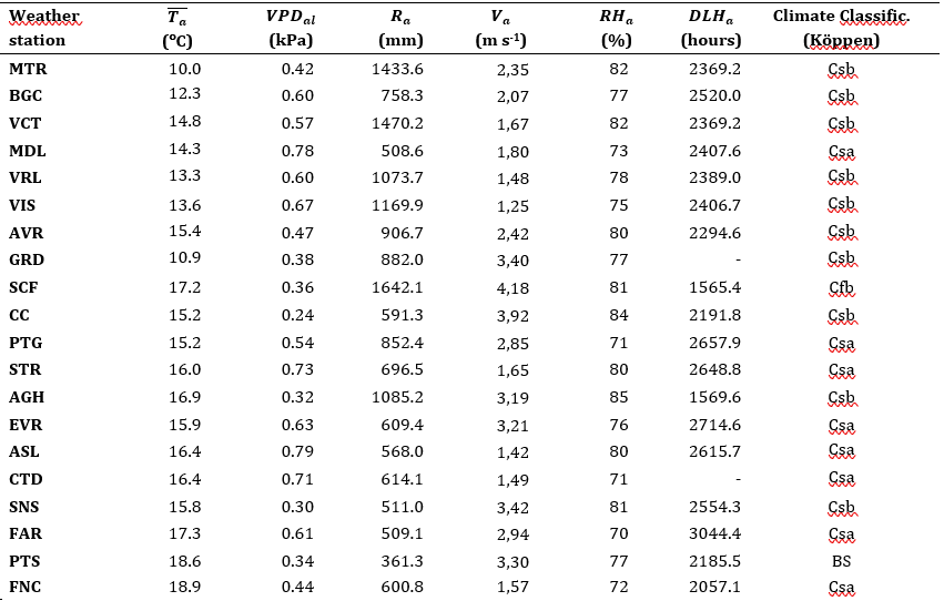
Climate types and subtypes based on the Climate Classification of Köppen reflect the territory's climate diversity. For each of the 20 stations studied, table II presents normal values (1971-2000) of the most relevant climatic elements (mean temperature - 𝑇 𝑎 , air vapor pressure deficit - 𝑉𝑃𝐷 𝑎 , rainfall - 𝑅 𝑎 , wind speed at 2m height - 𝑉 𝑎 , relative humidity - 𝑅𝐻 𝑎 and daylight hours - 𝐷𝐿𝐻 𝑎 , followed by the corresponding climate types: Mediterranean climate with cool - Csb, or hot summer - Csa and semiarid climate - BS. Locations with the greatest 𝑇 𝑎 are found in the south and on the islands (only SNS has a 𝑇 𝑎 below 16(C) whereas the coldest stations are found in the north inland (10(C≤ 𝑇 𝑎 <14(C). The lowest 𝑅 𝑎 values were also found in the south, where rarely exceeding 700mm. The rainiest locations ( 𝑅 𝑎 > 1000mm) are in the nothern Portugal (MTG, VCT, VRL, and VIS) and in Azores (SCF and AGH). 𝑉 𝑎 exceed 10kmh-1 in three out of four island stations (SCF, AGH, and PTS) and in three coastal stations (CC, SNS, and FAR). According to the United Nations Convention to Combat Desertification (Cherlet et al., 2018) all but one location is in the Humid climate-zone (PTS, with BS climate-type, is the exception). Ten locations have Csb climate (four on the continental coast, five in the northern or central-northern interior, and one in the Azores archipelago), eight have a Csa climate (two coastal locations, five inland, mainly in the central and southern regions, and one in the Madeira archipelago), one with a Cfb climate (SCF/Azores) whereas PTS/Madeira with a dry climate (BS).
Reference evapotranspiration (ETo) estimation methods
Monthly and daily values of climatic elements measured at 20 selected meteorological stations were used to estimate Reference Evapotranspiration (ETo). Normal monthly values (1971-2000) were used from all the stations. Monthly and daily values for 2019 and 2020 were used from two locations only (AVR and EVR). All data relating to AVR were obtained from one weather station whereas records for EVR were provided by two different stations (one located in the city centre, operational until the beginning of this century and the other on the outskirts of the city, providing data afterward).
Both monthly and daily ETo were estimated by PM and HS methods. As recommended by FAO, the former is taken as the standard method (Allen et al., 1998):
 (1)
(1)
where Rn is the net radiation at crop surface (MJ m−2 day−1), G is the soil heat flux density (MJ m−2 day−1), T is air temperature at 2 m height (◦C), u2 is the wind speed at 2m height (m.s−1), es-ea is the saturation vapour pressure deficit (kPa) (saturation vapour pressure minus actual vapour pressure), ( is the slope of the vapour pressure curve (in kPa (C-1) and ( the psychometric constant (kPa ◦C−1). To solve Eq. (1), standard meteorological records of solar radiation or sunshine duration (daylight hours), minimum, maximum and mean air temperature, air humidity and wind speed were required. Whether for calculating different parameters or overcoming a lack of data, the recommendations proposed by Allen et al. (1998) were followed. All requirements for meteorological data approval have been met. Latitude, altitude and height at which the wind speed was measured were the metadata considered.
The Hargreaves-Samani equation (Hargreaves & Samani, 1985) was recommended by Allen et al. (1998) whenever data required in the PM equation (moisture, wind, and/or radiation) are missing:
 (2)
(2)
where T, Tmax and Tmin (all expressed in (C) are, respectively, the mean, maximum and minimum temperatures of the time base used (daily or month), Ra is the extra-terrestrial radiation at the latitude, month and hemisphere considered (MJ m-2 day-1), ( is the latent heat of vaporization (MJ Kg-1) for the mean air temperature T ((C), Krs ((C 0.5) is the radiation coefficient (=0.17(C -0.5, by default) and 0.0135 is a factor for conversion from US to international units.
Analytical procedure
Annual, monthly and daily ETo values obtained by applying both PM and HS (with Krs=0.17) methods were compared. Linear regressions (y=bo+b1x, where y is ETo(PM), x is ETo(HS), bo and b1 are the intercept and slope, respectively) established between series of monthly or daily ETo values estimated by the two methods for each of the twenty locations. Goodness-of-fit was assessed using R2 (coefficient of determination), RMSE (the root mean square error) and RE (relative error):
 (3)
(3)
 (4)
(4)
 (5)
(5)
where ETo(PM)I and ETo(HS)I (i = 1, 2, . . . , n) represent pairs of values of ETo estimated using PM and HS equations, respectively, 𝐸𝑇 𝑜(𝑃𝑀) and 𝐸𝑇 𝑜(𝐻𝑆) are the respective mean values and no is the number of days used in the assessment.
Other regressions with lines forced to pass through the origin of the axes (y=b1x, where y, x and b1 have the same meaning) were also established between the same data series. Parameters of goodness-of-fit (R2, RMSE, and RE) were recalculated. Their values, naturally less favorable, are not comparable with those for the two-parameter lines. HS equation was then calibrated against PM equation. For this purpose, Krs coefficient was recalculated by multiplying the standard value (0.17) by the slope of the trend (straight) line obtained by regressions ETo(PM) = b1 ETo(HS). This procedure was suggested by Rodrigues and Braga (2021). The use of new Krs values should allow the HS method to replace the PM, whenever the scarcity of meteorological or climatic data is an obstacle and the correlation between the values obtained by the two methods is high. The Analysis ToolPak (Excel) software was used to analyze data related to the regressions performed.
The results obtained by comparing the two methods (differences, correlation, etc.) were evaluated and discussed based on the climatic factors that mostly influence the climate in Portugal: proximity to the sea (here measured by mean annual temperature ranges referred to 30 consecutive years) and elevation. Wind speed was also considered as a factor, either due to the importance it has in ETo calculations using the PM method, or due to the relevance given to several studies found in the literature, as mentioned above.
Results
Annual and monthly reference evapotranspiration (ETo)
1.1. Annual values of evapotranspiration (ET)
The annual ETo values obtained by applying the two methods from normal values (1970-2000) are shown in table III. Values estimated by PM method for the 20 stations considered ranged from 781mm (CC) to 1191mm (EVR) whereas those estimated by HS method ranged from 667mm (CC) to 1256mm (ASL). Unsurprisingly, the greatest values for ETo (above 1000mm per year) obtained by both methods were generally found in regions with hot summers (Csa) whereas the lowest (less than 950mm) were recorded where summer is cool (Csb and Cfb). Even so, this trend is more visible in the results obtained by the PM method than by the HS method.
Table III Mean annual values of ETo (PM and HS methods) obtained from climatic normal data (1971-2000).
| Weather stations | Methods | |
| HS (mm year-1) | PM (mm year-1) | |
| MTR | 865.6 | 863.4 |
| BGC | 1046.6 | 1004.5 |
| VCT | 1014.4 | 935.6 |
| MDL | 1199.1 | 1103.0 |
| VRL | 1053.9 | 936.6 |
| VIS | 1134.6 | 946.8 |
| AVR | 937.8 | 960.9 |
| GRD | 850.5 | 873.1 |
| SCF | 817.5 | 874.1 |
| CC | 666.9 | 781.0 |
| PTG | 1027.3 | 1063.9 |
| STR | 1189.4 | 1080.1 |
| AGH | 801.7 | 821.9 |
| EVR | 1124.6 | 1191.0 |
| ASL | 1255.6 | 1094.3 |
| CTD | 1201.3 | 1099.7 |
| SNS | 762.4 | 899.0 |
| FAR | 1110.7 | 1183.2 |
| PTS | 860.2 | 960.5 |
| FNC | 975.5 | 970.8 |
In half of the locations studied (MTR, BGC, VCT, MDL, VRL, VIS, STR, ASL, CTD, FNC) ETo(HS)>ETo(PM). ETo(HS)<ETo(PM) in the others. Absolute differences were relevant (> 100mm) in VRL, VIS, CC, ASL, CTD, STR, SNS, and PTS, and only residual (< 5mm) in MTR and FNC. These differences seem to be relatively independent of the climate type/subtype defined by Köppen for each of the 20 locations, that is, the maximum monthly temperature in the summer period (Csb vs. Csa) does not seem to determine the sign of the difference in the results of each method. In fact, ETo(HS)>ETo(PM) in half of the stations with Csb climate and in five out of eight locations with a Csa climate. Neither precipitation regimes nor annual precipitation seem to influence the direction of such differences: e.g., in both the wettest station (SCF, with Cfb climate) and in the driest (PTS, with BS climate), ETo(HS)> ETo(PM).
Figure 2 highlights the combined influence of mean annual thermal amplitude ( 𝑇𝐴 𝑎 ), mean annual wind speed ( 𝑉 𝑎 ) and elevation on the differences between the annual ETo values obtained by the two methods. In general, ETO(HS)< ETO(PM) whenever 𝑇𝐴 𝑎 are smallest (usually in coastal or insular areas) and 𝑉 𝑎 are greatest (≥ 2-2.5ms-1). Otherwise, the values obtained by the HS method overestimated those found by the PM method whenever 𝑇𝐴 𝑎 are greatest (generally > 10(C) and 𝑉 𝑎 are smallest (< 2 ms-1 in most cases). Only in three coastal locations (FNC, ASL, and VCT), all with 𝑉 𝑎 < 2ms-1, ETo(PM) was not underestimated. In ASL and VCT (with 𝑇𝐴 𝑎 similar to those observed in most inland locations) there was even a clear overestimate of the ETO calculated by the PM method. The only inland locations where ETo was underestimated, were those with 𝑉 𝑎 > than 2-2.5ms-1 (GRD, EVR, and PTG). Finally, elevation does not seem to have the same influence as each of the factors above does (locations at approximate altitudes show different trends). When elevation was evaluated as a factor associated only with atmospheric pressure variation (and not associated with temperature variation), ETo estimates using the PM method were based on sea level (( = 0,067 kPa◦C−1). In this context, the natural and consequent increase of ETo would range from about 15-17mm at MDL, VRL, VIS, CTD, and EVR (all located between 200 and 500m) to about 40mm at GRD and MTG (both located at about 1000m). If in these last two locations, this would mean an underestimate of ETo (PM) obtained by HS method and a relevant approximation between values in the cases of BGC and PTG.
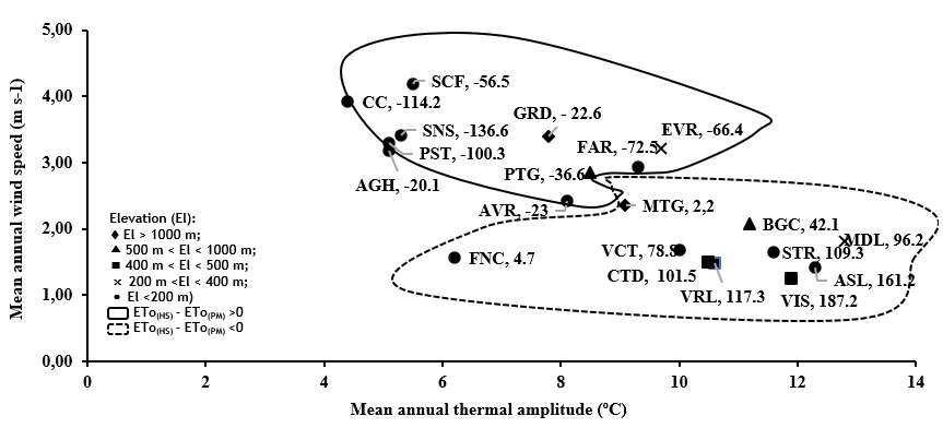
Fig. 2 ETo(HS) - ETo(PM) values as a function of wind speed and thermal amplitudes (mean annual values) for the 20 meteorological stations.
Figure 3 shows the influence of each of these factors (thermal amplitude, wind speed and elevation) on annual ETo(HS)-ETo(PM). For larger 𝑇𝐴 𝑎 reference ETo is overestimated whereas smaller ones underestimated it (fig. 3a). Despite the level of significance of the regression (p-value <0.05), the goodness-of-fit is just fair (R2=0.68). For thermal amplitude values close to 8(C, the differences were minimal. The results obtained by the two methods are very different for locations near the sea level, tending to be closer as the station elevation increases (except for VIS) (fig. 3b). Differences did not exceed 50 mm for stations located at more than 500m (4 out of 20). At elevations < 100mm, | 𝐸𝑇 𝑜 𝐻𝑆 − 𝐸𝑇 𝑜(𝑃𝑀) | ranged from 5mm to 161mm. The relationship between| ??𝑇 𝑜 𝐻𝑆 − 𝐸𝑇 𝑜(𝑃𝑀) |, and 𝑉 𝑎 was well-described (R2= 0.782) by a straight line (with a negative slope). The statistical relevance of this trend is also significant (p-value < 0.1) (fig. 3c). This means that the HS method tends to underestimate the values obtained by PM under windier conditions and overestimate them under less windy conditions. The 𝑉 𝑎 corresponding to a zero-difference was 2.61 ms-1 (a reasonable criterion to distinguish, for this purpose, windy locations from non-windy locations).
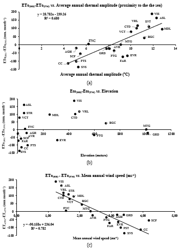
Fig. 3 ETo(HS)- ETo(PM) vs.: (a) Mean annual thermal amplitude ( 𝑇𝐴 𝑎 ); (b) elevation and (c) mean annual wind speed ( 𝑉 𝑎 ) for the 20 weather stations studied.
The annual ETo(HS) values obtained by both methods from data recorded in AVR and EVR during 2019 and 2020 were also different (data not shown). As with normal data, those obtained in AVR by ETo(HS) underestimated (by approximately 15-20mm) those found by the PM method. On the contrary, ETo(HS) > ETo(PM) in both years, with differences greater than 100mm. The relocation of the weather station in EVR (to a less windy location) could explain this fact, reinforcing the importance of wind speed in the differences between the ETo obtained by the two methods.
1.2. Monthly values of Evapotranspiration (ETo)
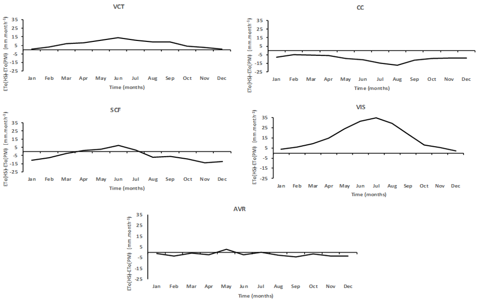
The variations in ETo values throughout the year estimated by both methods largely reflect the central influence of temperature on the evapotranspiration process: minimum values in December/January and maximum values in July/August at these latitudes. Winter minimum values of 20-30 mm are common in most places (ASL, FAR, and insular locations were exceptions). In summer, ETo often reached monthly values close to 200mm in the inland, mainly south, whereas on the islands and on two coastal locations (CC and SNS) they never exceeded 120mm. The differences ETo(HS)- ETo(PM) also vary throughout the year (fig. 4), generally reaching the greatest magnitudes during the hottest period. The exceptions were PTG, FAR, and SCF, where the differences were more noticeable in the autumn-winter period, and AVR, where they never exceeded five mm.
Monthly ETo(PM) values were always lower than ETo(HS) in VCT, VRL, VIS, ASL, CTD, and STR (the six least windy locations) and always greater at CC, SNS, FAR, and PTS (four of the windiest locations) (eg., fig. 4a and 4b, respectively) . In the other locations, the differences are negative in one part of the year and positive in another (eg., fig. 4c). ETo (HS) - ETo (PM) exceeded 20mm in at least one month at MDL, VRL, VIS, STR, ASL, and SNS (eg., fig. 4d). At MTG, AVR, GRD, PTG, FAR, AGH, FNC, the differences between monthly values never exceeded 10 mm (eg., fig. 4e).
2. Correlations between monthly or daily values obtained by HS and PM methods
2.1 From normal monthly values
Monthly values of ETo(PM) were plotted against those of ETo(HS). The regression equations and goodness-of-fit parameters are shown in table IV. The linear correlations were very significant in all cases (p-value <0.01) and the goodness-of-fits were very high (R2 was around 0.98 and 0.97 in the island locations and SNS, and ≥0.99 in the others). Although unsurprisingly the RMSE and RE values in most cases increased significantly when the line was forced to cross the origin, the R2 values remained quite high (only in SCF R2<0.97). Decreases were greater than 50% in 10 locations (VCT, VRL, VIS, STR, ASL, CTD, SNS, MDL, CC, and PST) and only residual (<5%) in 5 (GRD, SCF, PTG, AGH, and FNC).
When in the equation forced to pass through the origin the b1 values were > 1 (VCT, MTL, VRL, MDL, BGC, VIS, STR, ASL, CTD, FNC, and especially in VIS), the Krs used (0.17(C-0.5) proved to be excessive; when b1 <1 (PTG, EVO, FAR, PTS, SCF, AGH, and especially in SNS, and CC) the Krs values were naturally deficient. In AVR and in GRD, the Krs value proved to be adequate. The HS method can then be calibrated by applying the new Krs values to the HS equation. For the places farthest from the sea, Krs values ranged from 0.155(C -0.5 (MDL) to 0.177 (C-0.5 (EVR) whereas on the mainland coast, the range of values was wider (from 0.149(C -0.5 at ASL to 0.201(C -0.5 at CC). At island stations, corrected Krs values ranged from 0.169 (C -0.5 (FNC) to 0.188 (C-0.5 (PTS). The lowest value was registered in VIS (0.14(C -0.5) (fig. 5).
A significant (p-value <0.05) and an acceptable (R2=0.69) linear correlation was found (fig. 6a) when the influence of 𝑇𝐴 𝑎 on the variation of the Krs coefficient was tested. The quality of regression fit was considerably improved when only mainland locations were considered (R2=0.81). In a hypothetical isothermal environment (not verifiable in this climate-type), Krs would be between 0.21 and 0.23, depending on the established regressions. As thermal amplitudes increase (increase supposedly associated with increasing distance from the sea) the value of Krs decreases. Adjusted Krs values in insular territories are visibly lower than those obtained in coastal sites with similar thermal amplitudes. In addition, W-E transects without a coherent trend (fig. 3a) suggest that other factors may also be required to better calibrate Krs.
Table IV Linear regressions between values estimated by PM (y-variable) and PM (x-variable) methods for (20) weather stations (equations, R2 - coefficient of determination, RMSE - root mean square error and RE - relative error).
| Weather station | y =b1x +bo | y=b1x | ||||||
| Equation | R2 | RMSE | RE | Equation | R2 | RMSE | RE | |
| MTG | y =0.921x+5.509 | 0.996 | 2.705 | 3.760 | y =0.977x | 0.991 | 3.929 | 5.575 |
| BGC | y =0.929x+2.646 | 0.997 | 2.675 | 3.196 | y =0.952x | 0.996 | 3.001 | 3.616 |
| VCT | y =0.905x+1.478 | 0.999 | 1.312 | 1.683 | y =0.919x | 0.999 | 1.465 | 1.886 |
| MDL | y =0.894x+2.559 | 0.993 | 4.431 | 4.821 | y =0.913x | 0.993 | 4.622 | 5.066 |
| VRL | y =0.871x+1.545 | 0.997 | 2.524 | 3.234 | y =0.884x | 0.997 | 2.648 | 3.410 |
| VIS | y =0.791x+4.108 | 0.999 | 1.579 | 2.001 | y =0.824x | 0.996 | 2.551 | 0.273 |
| AVR | y =0.978x+3.650 | 0.997 | 1.707 | 2.131 | y =1.0017x | 0.995 | 2.242 | 0.235 |
| GRD | y =0.927x+7.032 | 0.993 | 3.356 | 4.613 | y =1.0002x | 0.985 | 4.938 | 0.580 |
| SCF | y =0.833x+16.092 | 0.972 | 4.158 | 5.708 | y =1.0312x | 0.907 | 7.635 | 10.863 |
| CC | y =1.106x+3.622 | 0.985 | 2.850 | 4.379 | y =1.163x | 0.982 | 3.118 | 4.824 |
| PTG | y =0.962x+6.288 | 0.994 | 3.907 | 4.407 | y =1.016x | 0.990 | 5.062 | 5.817 |
| STR | y =0.905x+0.349 | 0.996 | 2.996 | 3.328 | y =0.907x | 0.996 | 3.000 | 3.336 |
| AGH | y =0.896x+8.605 | 0.984 | 3.305 | 4.841 | y =1.005x | 0.996 | 4.714 | 7.018 |
| EVR | y =0.993x+6.198 | 0.989 | 5.454 | 5.495 | y =1.044x | 0.969 | 6.219 | 6.368 |
| ASL | y =0.882x-1.046 | 0.997 | 2.295 | 2.516 | y =0.874x | 0.997 | 2.345 | 2.565 |
| CTD | y =0.891x+2.482 | 0.998 | 2.256 | 2.462 | y =0.909x | 0.998 | 2.573 | 2.827 |
| SNS | y =1.198x-1.163 | 0.983 | 3.555 | 4.745 | y =1.181x | 0.982 | 3.576 | 4.765 |
| FAR | y =0.954x+10.266 | 0.997 | 2.341 | 2.374 | y =1.046x | 0.986 | 4.858 | 5.017 |
| PTS | y =1.006x+7.896 | 0.979 | 3.505 | 4.379 | y =1.105x | 0.969 | 4.311 | 5.441 |
| FNC | y =0.963x+2.645 | 0.981 | 3.223 | 3.984 | y =0.993x | 0.980 | 3.309 | 4.102 |
Also a significant (p-value <0.05) and acceptable (R2=0.72) linear correlation was found when Krs values are plotted against 𝑉 𝑎 (fig. 6b). When only mainland locations were considered the goodness-of-fit also increased (R2= 0.87). The best fit between Krs and wind speed is not surprising, as this already explained the variation of ETO(HS)-ETO(PM) (annual values) better than any other parameter. For mainland locations, in the absence of wind, Krs=0,123(C-0.5 (0.113 < Krs < 0.133, with 95% of confidence), a useful value for predicting Krs as a function of wind speed (T-test for (=0.05). Finally, when the effect of atmospheric pressure is removed, the Krs values increase very slightly (only at the two highest locations do the increments exceed 0.005(C-0.5).
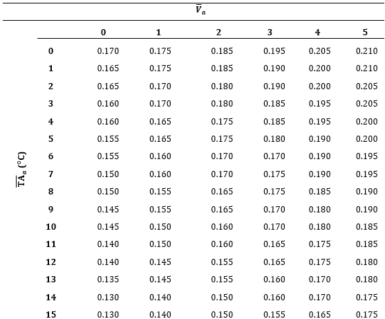
If a multiple linear regression is used, with 𝑉 𝑎 and 𝑇𝐴 𝑎 as independent variables (predictors), more significant (p-value <0.05) and better correlations (R2 equal to 0.79 or to 0.91 when all locations or only mainland locations were considered, respectively) were found (fig. 7). P-values for both independent variables were < 0.05together then. In short, Krs is better explained by both variables jointly. Table V presents Krs values (approximated to 0.005(C-0.5) for different combined values of 𝑉 𝑎 and 𝑇𝐴 𝑎 (both approximated to units).
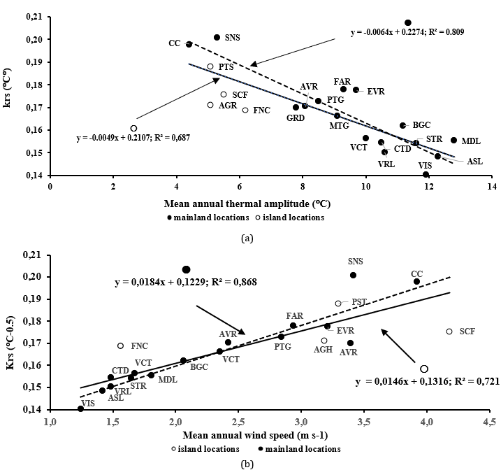
Fig. 6 (a) Krs-values = f ( 𝑇𝐴 𝑎 ) and (b) Krs-values = f ( 𝑉 𝑎 ) for 20 weather stations in Portuguese territory. R2 - coefficient of determination.
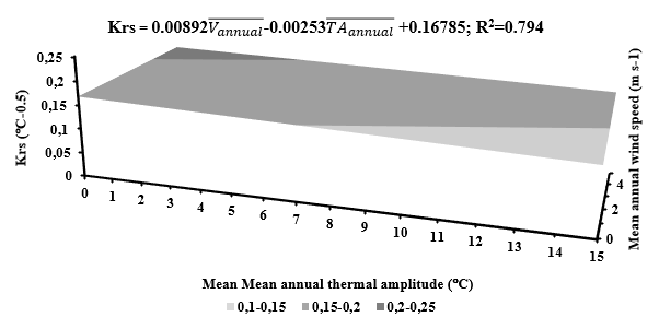
Fig. 7 Krs-values estimated (by multiple regression) as a function of both (normal) annual thermal amplitude and wind speed values, for 20 weather stations in Portuguese territory. R2 - coefficient of determination.
Table V Krs values (in (C -0.5; approximation: 0.005(C -0.5) fitted for different combination of mean annual thermal amplitude (TA 𝑎 ) and mean annual wind speed ( 𝑉 𝑎 ), using the equation: Krs = 0.00892 𝑉 𝑎 -0.00253 𝑇𝐴 𝑎 +0.16785.
2.2. From monthly values recorded in 2019 and 2020
Correlations between the monthly ETo values estimated by the two methods for 2019 or 2020 were also good, whether the trend lines found has been forced to pass through the origin or not (R2 was always greater than 0.97) (fig. 8). Correlations between the average values for AVR referred to these two years were not significantly different (p≥0.05) from those found when normal values were used, but those for EVR were significant (p<0.01). Consequently, similar Krs values were obtained (0.17-0.171 in any case) in AVR, but not in EVR (Krs ( 0.16 in the two years studied and around 0.18 for the 30 years considered).
2.3 From daily values recorded in 2019 and 2020
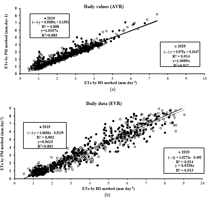
Correlations between the daily values for to AVR and EVR obtained by both methods were also significant (p-value <0.01). Goodness-of-fit was also high (R2(0.90) for any of the years considered (2019 or 2020), allowing us to use the HS method instead of PM on a daily basis as well (fig. 9). RMSE for AVR ranged from 0.37 mm day-1 (2019) to 0.41 mm day-1 (2019) whereas for EVR it ranged from 0.77 mm day-1 (2020) to 0.80 mm day-1 (2019). When the regression line was forced to pass through the origin (bo=0), R2 did not drop substantially (also around 0.90). The decrease in RMSE resulting from using this relationship to estimate ETo(PM) from ETo(HS) was around 10% in EVR for 2020. The default value of Krs used by default (=0.17) was overestimated in EVR ((0.16) whereas in AVR it seemed to be adequate. Estimates for AVR were similar to those found for monthly estimates (from both normal data and the data for 2019 and 2020), whereas for EVR they were clearly smaller than those obtained when monthly data were used.
When comparing the daily values separately for each of the two semesters (April-September and October-March) the R2 values decreased substantially in both locations, to around 0.78 in both semesters in the case of EVR, and to 0.84 and 0.59, respectively in the hottest and coldest semester, in the case of AVR (data not shown) The Krs for both semesters were similar in AVR ((0.17), but not in EVR (0.164 for the warmer semester and 0.139 for the other).
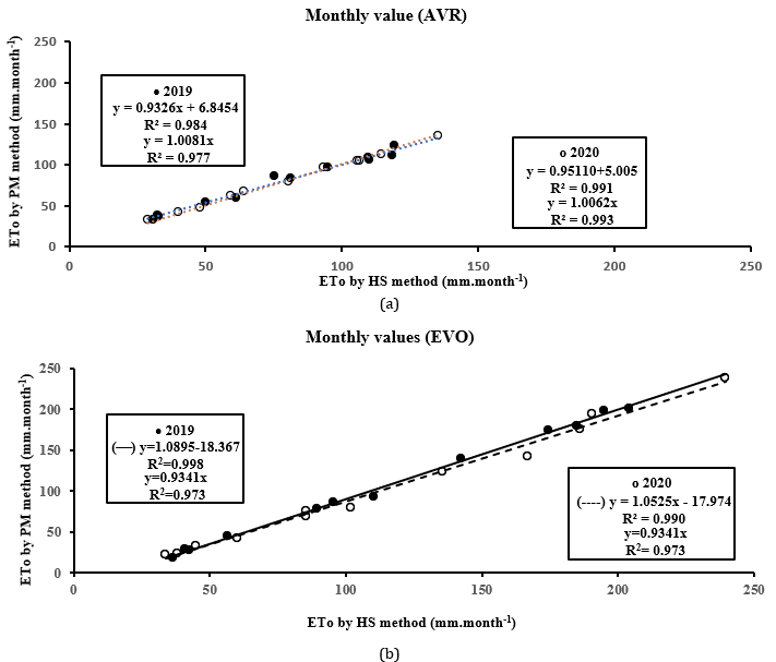
Fig. 8 ETo(PM) vs. ETo(HS) (linear regressions) with monthly values for 2019 (() and 2020 (() in (a) AVR and (b) EVR. Only the straight lines y=b1x+bo are shown: 2019 ( () and 2020 ( _ _ _ ). R2 - coefficient of determination.
Discussion
Regardless of the time scale used (monthly or daily), the (good) linear fit quality obtained in this study for the relationship between ETo values estimated by PM and HS methods is consistent with results found by various authors for different climatic conditions. Thus, even in Mediterranean-type climates (Csa and Csb, according to the Köppen Classification), the ETo values obtained by the HS method are also good predictors of those obtained by the reference method (PM method), thus contributing to the widespread use of the former, whenever climatic/meteorological data needed to perform the PM method are missing, unreliable or when maximum rigor is not required. Since the studied area (Portugal) is considered humid by the classification proposed in the World Atlas of Desertification for the aridity index (Cherlet et al., 2018), that is, 𝑃 𝑎 ≥ 0.65 𝐸𝑇 𝑜 ̅ in all but one of the studied sites, the use of ETo estimated by the HS method as a predictor of that estimated by the PM method can thus be extended to areas outside those that were initially most associated with its good performance (semi-arid and arid areas, according to the aridity index). However, it does not seem that this association should be used as a criterion of suitability without the dry/wet terminology being adequately quantified and consequently, agreed upon.
The differences found between the values obtained by the two methods reflect the relevance they attribute to the climatic factors associated with each parameter used. In addition to the influence of the proximity of the sea on the calibration of the HS equation, that of the wind speed was also important (perhaps as, or more, influential than the distance to the sea). Reference to the influence of wind speed had already been made by Allen et al. (1998) in the differences obtained between the two methods and by Martinez-Cob & Tejero-Juste (2004) in the calibration of the HS equation. Contrary to what the latter authors suggested for regions relatively similar to those studied in this work, our results show that local calibration of the HS equation is just as necessary in windy areas as in areas that are not windy. On the other hand, elevation/altitude, a relevant climatic factor in Portugal, seems to have much less influence on the correspondence between both methods than other factors. Due to the importance attributed by the HS method to air thermal amplitude, the importance of hotter summers due to increased distance from the coastline is reduced, thus attenuating the effect of altitude on the ETo estimate. This seems to be the case for inland locations in mainland Portugal such as VIS, VRL or BGC (Csb climate-type, due to the altitude), which presented greater ETo values (HS) than other locations with Csa climate-type.
Although the two highest Krs values were estimated for two coastal stations (SNS and CC), the proximity to the sea as a predominant factor in the variation of Krs, as proposed by Hargreaves (1994) and later by Allen et al. (1998) (ranging from 0.16(C-0.5 to 0.19(C-0.5 respectively for inland or coastal regions), was not confirmed, at least not with the relevance that those authors attribute to it in the recalibration of the HS equation. The low value of Krs (0.146) estimated for ASL, just greater than that recorded in VIS (0.145), an inland location, suggests the importance of thermal amplitude in low windy places, even close to the sea, as is the case (ASL it is the only monitored continental coastal site, facing west, that presented a Csa climate). In short, in parallel with the decrease in Krs with increasing in air thermal amplitude (fig. 6a) also suggested by other authors, e.g. Gavilan et al. (2006) and Raziei and Pereira (2013), the increase in Krs with wind speed (fig. 6b) should be considered, suggesting a combined analysis of the influence of both factors rather than separately. In this work, it was possible to reasonably approximate the values obtained by both methods when using both 𝑉 𝑎 and 𝑇𝐴 𝑎 as predictor variables in a multiple regression to estimate Krs (dependent variable) and thus find a better calibration solution for the HS equation, increasing the usefulness of the method. The frequent unavailability of wind speed values can be a major drawback when running this regression. However, the problem can be mitigated by using annual average values instead of values associated with shorter time scales.
In summary, the findings suggest a calibration factor for each location, which may be expensive and not feasible. Identifying locations with analogous geophysical characteristics and assigning them a calibration factor (Krs) for the HS equation can be a good solution. The values obtained could then be applied to regions with similar characteristics. This would involve conducting similar studies to establish Krs values for each classifiable area or region, which would require extensive sampling.
When we include the Krs values of the four island locations, the fit of the data becomes worse, whether we consider the wind factor or air thermal amplitude separately or jointly (using multiple regression). This is probably because they are, among the windiest places, those with the greatest 𝑇 𝑎 . The mild winters on these islands result in very high average annual temperatures, which can significantly lessen the impact of the sea's proximity on the results obtained by the HS method (Tmax-Tmin). Furthermore, the greater air humidity on the islands (with mean annual vapour pressure always greater than 1.65kPa and very low air saturation deficits) can reduce the role of wind in the differences found, and therefore in the value of Krs.
Stefano and Ferro (1997) and Hargreaves and Allen (2003) also found a decrease in the quality of the fit when the data considered is daily rather than monthly. These authors explain this decrease by the increased influence of the temperature range caused by frontal movement and rapid variations in wind speed and cloudiness. The RMSE values obtained AVR were lower than those found by Gavilán et al. (2006) in locations in southern Spain, while those found in the EVR were of the same order of magnitude. If compared with those obtained by Rodrigues and Braga (2021) for the same location (EVR), the RMSE values found in this work were slightly lower. The comparison between the Krs values obtained for both locations (AVR and EVR) with monthly and daily values recorded in 2019 and 2020 suggests that Krs is independent of the time base used, that is, that Krs is a conservative factor. However, the Krs EVR values obtained from values (daily or monthly) recorded in these two years were lower (by about 0.01-0.02) than those obtained with normal data (1970-2000), while those obtained in AVR remain constant (around 0.17). The relocation of the station representative of a given location may imply a change in the microclimate (for example, from an urban area to the periphery, as in EVR) and, therefore, a variation in Krs values. Naturally, a larger sample will be needed to confirm this hypothesis or not.
The Krs values were similar in the two semesters in the case of AVR but different in the case of EVR.The assumption that different calibration factors depend on the semester considered was also advanced by Borges and Mendiondo (2007) in a study carried out in the Jacupiranga River Basin (Brazil). The intensity with which meteorological phenomenology (frontal movement) influences the calibration of the HS equation on a daily basis (Hargreaves & Allen, 2003) can also change considerably from semester to semester, a fact that is more common the closer the regions under study are from mid-latitudes.
In short, the Krs calibration factor should not be generalizable for a given region, rather it should consider important factors and/or climatic elements in each location. Thus, the need for prior local calibration proposed by several authors seems appropriate. Furthermore, the behaviour of different factors on sub-monthly time scales (e.g., daily) in the calibration of the HS method for these same locations requires a more detailed analysis.
Conclusions
In climates with Mediterranean characteristics (namely Csa and Csb climatic types), estimates of ETo obtained by the HS method are very good predictors of those obtained by the reference method adopted and recommended by FAO (PM method), regardless of the time base used (normal monthly data, monthly or daily values). Even so, the quality of fit was lower when daily data, isolated or aggregated into semesters, are used. However, the correlations between daily values, especially when separated between opposite semesters (cold and hot) seem to provide lower quality correlations.
These results also make the HS equation easy to calibrate, using the Krs value for this purpose. Corrected Krs values depend more on wind speed (annual mean) than on factors such as proximity to the sea or elevation. A significant and good correlation was obtained when Krs was plotted against both mean annual wind speed and mean annual thermal amplitude as independent variables (multiple regression). This allows the Hargreaves-Samani equation to be successfully calibrated as a function of combined values of these two independent variables. The hypothesis of a constant Krs value for each location, regardless of the time base used, has not been fully confirmed.

