ARTIGOS

 

Linear Mixed Modelling of Cone Production for Stone Pine in Portugal

Modelação da produção de pinha em pinheiro-manso em Portugal recorrendo a modelos lineares mistos

Modélisation de la production de cônes de pin parasol au Portugal avec des modèles mixtes linéaires

 

*Abel Rodrigues, **Giovani L. Silva, ***Miguel Casquilho, ****João Freire, *Isabel Carrasquinho e *****Margarida Tomé

*Senior Researcher, Instituto Nacional de Investigação Agrária e Veterinária, IP. Unidade Estratégica de Investigação de Sistemas Agrários e Florestais e Sanidade Vegetal. Quinta do Marquês, 2780-159 OEIRAS. E-mails: abel.rodrigues@iniav.pt; isabel.carrasquinho@iniav.pt;

**Professor, Centro de Estatística e Aplicações and Dept. Matemática, Instituto Superior Técnico, Universidade de Lisboa. Av. Rovisco Pais 1, 1049-001 LISBOA. E-mail: giovanni.silva@tecnico.ulisboa.pt

***Professor, Centro de Processos Químicos, Instituto Superior Técnico, Universidade de Lisboa. Av. Rovisco Pais 1, 1049-001 LISBOA. E-mail: mcasquilho@tecnico.ulisboa.pt

****Research grant-holder

*****Full Professor, Centro de Estudos Florestais. Instituto Superior de Agronomia. Universidade de Lisboa, Tapada da Ajuda, 1349-017 LISBOA. E-mails: joaofreire71@gmail.com; magatome@isa.ulisboa.pt

 

ABSTRACT

This study aimed to model the cone production weight of stone pine (Pinus pinea L.) trees using two approaches: classic linear mixed modelling and Bayesian mixed modelling. The field data were collected in the Setúbal Peninsula, the main production area in Portugal, where 51 plots for monitoring cone production per tree during three production periods (2004–2005, 2005–2006 and 2006–2007) were set up. Linear mixed models with a random intercept term were fitted to the whole dataset (416 trees) for the three production periods. Clustered longitudinal mixed models, under a Bayesian approach with random terms related to intercept, time slope and nested effects, were fitted to a subset of the global dataset (9 plots and 76 trees), corresponding to the plots where production data for all trees in the three years were available. The selected models included, as independent variables, crown width, basal area per hectare, tree height and accumulated rainfall in the five-year periods, prior to cone collection. Despite the small period considered in this study, the Bayesian analysis proved to be useful for calculations with smaller samples, and it was indicative about the tree and plot biometric complex dynamics, subjacent to cone production.

Key words: stone pine, cone production, mixed models, Bayesian analysis, clustered longitudinal data

 

RESUMO

Este estudo visou a quantificação da produção de pinha em povoamentos de pinheiro-manso (Pinus Pinea L.) segundo duas abordagens: utilização de modelos mistos clássicos e modelação Bayesiana longitudinal mista. Os dados de campo foram obtidos na Península de Setúbal, a principal zona produtora em Portugal, onde se instalaram 51 parcelas para quantificação da produção de pinha durante três períodos de produção (2004-2005, 2005-2006 e 2006-2007). Os modelos mistos lineares com um termo de interceção aleatório, correspondente a cada parcela, foram ajustados a um conjunto de 416 árvores, para os três períodos, independentemente do período de produção ou de não disponibilidade de alguns dados, devido a dificuldades logísticas no terreno. Os modelos mistos longitudinais, ajustados por metodologia Bayesiana, com termos aleatórios associados à interceção, fator temporal e efeitos encaixados foram aplicados a um subconjunto de 76 árvores em 9 parcelas, para as quais estavam disponíveis os dados de produção para os três períodos de produção. Os modelos selecionados incluíram como variáveis independentes a largura das copas, a área basal por hectare, a altura das árvores e a precipitação acumulada nos períodos de cinco anos, anteriores à recolha das pinhas. Apesar do curto período abrangido por este estudo, a análise Bayesiana revelou-se útil para cálculos com amostras e indicativa sobre a dinâmica complexa do sistema árvore-parcela, subjacente ao processo de produção de pinha.

Palavras-chave: pinheiro-manso, produção de pinha, modelos mistos, análise Bayesiana, análise longitudinal agrupada

 

RÉSUMÉ

Cette étude visait à quantifier le poids de la production de cônes en peuplements de pin parasol (Pinus pinea L.), moyennant deux approches: modélisation mixte linéaire et modélisation Bayésienne mixte longitudinale. Les données de champ ont été recueillies dans la péninsule de Setúbal, la principale zone de production au Portugal, y étant préparées 51 parcelles pour l'observation de la production de cônes pendant trois périodes productives (2004-2005, 2005-2006 et 2006-2007). Des modèles mixtes linéaires avec un terme d'interception aléatoire, correspondant à chaque parcelle, ont été ajustés à l'ensemble des données (avec 416 arbres) pour les trois périodes productives, sans rapport avec l'année de production ou l'absence de données, en raison de problèmes logistiques dans le champ. Des modèles mixtes longitudinaux, sous une approche Bayésienne avec des termes aléatoires relatifs à l'ordonnée à l'origine, au facteur temps et aux effets imbriqués ont été ajustés à un sous-ensemble des données globales (9 parcelles et 76 arbres), correspondant aux parcelles où étaient disponibles des données productives pour tous les arbres dans les trois années. Les modèles sélectionnés ont inclus, comme variables indépendantes, la largeur de la cime, la surface basale par hectare, la hauteur de l'arbre et la précipitation accumulée dans la période de cinq ans antérieure à la récolte des cônes. Malgré la brièveté de la période ciblée dans cette étude, l'analyse Bayésienne s'est révélée utile pour les calculs avec des échantillons plus petits, et fut révélatrice quant à la complexe dynamique biométrique sur l'arbre et la parcelle, sous-jacente à la production de cônes de pin.

Mots-clés: pin parasol, cônes, modèles mixtes, analyse Bayésienne, données groupées longitudinales

 

Introduction

Stone pine (Pinus pinea L.) is a Mediterranean forest species with the highest rate of increase in area in Portugal since 1995, occupying approximately 176 thousand ha, about 6% of the total national forest area (ICNF, 2013). It represents the fifth largest forest area, mainly for kernel production. From the total forest area of this species, about 106,200 ha correspond to young pure plantations (ICNF, 2013). This large expansion is due to its good adaptability to high air temperatures and low rainfall in summer, typical of the Mediterranean climates and to the high economic value of the edible kernels. Spain is also another big stone pine producer with an area of about 60% of the world's stone pine woodland and pine nut production (CALAMA et al., 2008). Together the two countries account for about 75% of stone pine's world area. Portuguese average cone production was 193 kg ha^-1 in 2006 (ICNF, 2013).

Stone pine stands are also less sensitive to diseases and pests comparatively to other Mediterranean pine species, particularly Monochamus galloprovincialis vector of the pine wood nematode (Bursaphelenchus xylophylus), the agent of pine wilt disease recorded in Portuguese maritime pine stands since 1999. This makes stone pine a potential candidate for the replacement of some attacked maritime pine forests.

Stone pine is a native species in Portugal with the Setúbal Peninsula, in the southern coast, being its main concentrated area with more than 50% of national cone production (ICNF, 2013). Stone pine provides wood and non-wood products. Its main value comes from the nuts which are the most important edible product in Mediterranean forests (CARRASQUINHO et al., 2010). Less important, but still relevant, are the wood and resin productions.

Cone production per tree is a complex process depending on intrinsic and extrinsic factors to trees (CANÃDAS, 2000). There are genetic, hormonal and nutritional factors associated with tree age and health status. Site, climate and disturbances such as forest fire or diseases may also affect stand productivity. All these factors interact in complex patterns and processes, e.g.,flowering dynamics, easiness in cone detachment or yearly fluctuation of cone production per tree. In Portugal, long term empirical evidence suggests that cone yield follows a cycle of 7 or 8 years (CARRASQUINHO et al., 2010). Nut yield changes every year, and the annual number of flowers, related to the number of cone buds, depends on the winter conditions of the previous year. On the other hand, a plentiful flowering sinks organic and inorganic nutrients, allowing for less available resources to the trees in the following vegetative cycles, with lower diameter and crown growth (CANÃDAS, 2000).

A linear mixed model (LMM) is a parametric linear model that includes a continuous response variable and also random and fixed effects as independent variables, allowing the clustering of available data. The parameter estimation is based on maximum likelihood (ML) or restricted maximum likelihood (REML) theory (e.g., SEARLE et al., 2006), allowing to simultaneous estimation of fixed and random effects, under a proposed matrix structure for random variables and error terms. LMMs are primary fundamental tools with an untapped potential for forest modelling at large. LMMs allow to quantify the linear relationships (e.g., CANÃDAS, 2000; CALAMA, 2004; CALAMA and MONTERO, 2005; CALAMA et al., 2007) between stone pine cone production and tree and plot biometrical and environmental covariables. These models, by dividing the residual variance into different components, facilitate a discrimination of different sources of stochastic variability, related to possible levels of clusters, repeated measures and longitudinal analysis. Examples of these covariables are: diameter at breast height, crown diameter and height, tree height, average distance between trees, total number of trees per hectare or basal area by hectare. Linear mixed models can consider both classic (or frequentist) and the Bayesian statistical approaches. The Bayesian approach relies on the prior information about the model parameters, for which is considered a probability distribution, beyond the data information present on the likelihood, allowing to obtain the posterior distribution in order to make inference on the model parameters (e.g., PAULINO et al., 2003; GELMAN et al., 2006). We believe that the use of the Bayesian analysis for modelling cone production in stone pine is innovative compared to previous related studies.

Significant research work has been made on stone pine in the last 15 years concerning items as diameter increment (CALAMA and MONTERO, 2005; FREIRE, 2009), regional growth models (GARCÍA GÜEMES, 1999; CALAMA, 2004), variability of cone and seed production with geographical location and time by use of mixed models (CALAMA and MONTERO, 2005; CALAMA, 2004; FREIRE, 2009), empirical ecological type models for predicting stone pine cone production (CALAMA et al., 2008), stem form and tree volume (ALPUÍM et al., 2000; CALAMA and MONTERO, 2006) or effects of fertilization in stone cone production (CALAMA et al., 2007). This recent work has been carried out mainly in Spain, whereas for Portugal few generalized production models have been found in literature (FREIRE, 2009; CARRASQUINHO et al., 2010).

Regarding meteorological conditions, the most cone productive areas within a region of natural distribution are these in lower elevation, with warmer temperatures, free of extreme winter conditions and without lack of available water (CALAMA et al., 2008). Winter rainfall also explains temporal and spatial variability of flowering and fruiting processes in Mediterranean forests (KOENIG et al., 1996; MUTKE et al., 2005; CALAMA et al., 2008). Stone pine has a strong epinastic control based on two climatic years regarding the formation of buds and the primary growth, respectively (SUROVÝ et al., 2011). According to GONÇALVES and POMMERENING (2012), long term climate and production data would be necessary for each stone pine stand, to evaluate the influence on cone production by intrinsic and extrinsic factors.

Individual cone yield is linked to variables related to tree biometry, such as diameter at breast height (dbh) and crown diameter, up to advanced stages of cone production (CAÑADAS, 2000; MUTKE et al., 2000). Evidence indicates that trunk section just below the crown is well correlated with photosynthetic activity inducing leaf and cone production (CAÑADAS, 2000). For Spain, GARCÍA GÜEMES (1999), MUTKE et al. (2000) and CALAMA et al. (2008) pointed out that higher average cone yield both at stand or tree level was related to higher site index and also to covariables such as a lower number of trees or a higher basal area per hectare. The stand basal area is strictly associated to plot density and free space available for trees. CAÑADAS (2000) suggests dominant height of the hundred trees with the higher dbh in dominant strata per ha on regular stands as a parameter to evaluate site index in stone pine forests. GONÇALVES and POMMERENING (2012) for west-southern Portugal, grossly the same area of this study, point out that tree spacing and crown size are factors positively correlated with stone pine cone production. The tree spacing influence is probably associated with the light demanding nature of this species and with the competition for water and nutrients especially in conditions of low summer rainfall and low soil water and nutrient availability.

The present study is a sequence of the work made by CARRASQUINHO et al. (2010), on stone pine stands in Setúbal Peninsula. Our main objective is to obtain two independent kinds of linear mixed models, based on classic LMMs and Bayesian approaches, aimed to quantify the cone production per stone pine tree for the period of 2004-2007.

 

Materials and methods

Datasets and exploratory analysis

Under a joint initiative of the Portuguese "National Institute of Agrarian and Veterinarian Research" (INIAV), the Institute of Agronomy, the Portuguese Forest Service and local associations of forest owners, 51 stone pine field plots (Table 1) for measurement of cone production and several biometric variables were set up in 2004 and 2005. These plots are representative of the main stone pine Portuguese provenance region in the Setúbal Peninsula. The field work took place from 2004 to 2007. The plots had a circular shape, were typically even-aged and natural-regenerated. Plots with a maximum of 25 trees were 20 m radius and 30 m otherwise. The 14 variables measured or calculated were tree height (h), diameter at breast height (dbh), crown width (cw), basal area (g), crown height (ch), base crown height (bch), total number of trees per hectare (N_T), total basal area per hectare (G_T), dominant height (HD), dominant diameter (DD), crown area (CA), number of stone pine trees per hectare (N_SP), stone pine basal area per hectare (G_SP), and annual rainfall (R).

 

 

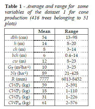
Five groups of trees were defined (CARRASQUINHO et al., 2010) depending on diameter at breast height: i) juvenile (dbh < 11 cm); ii) dominant vegetative growth (11 cm < dbh < 28 cm); iii) cone production phase I (28 cm < dbh < 46 cm); iv) cone production phase II (46 cm < dbh < 62 cm), and v) cone production phase III (62cm < dbh < 82 cm). Average yearly cone weight production by tree j in plot i (CWP_ij) was measured in trees belonging to the three productive phases. Unfortunately, due to practical reasons in the field, it was not possible to record cone production data for the three production years to all plots, and thus two distinct datasets were established, included in Table 1 and Table 2. Cone weight production was evaluated from datasets of 416 trees (Table 1) and 76 trees (Table 2) in the productive stages, belonging to 51 and 9 plots, respectively. The dataset 1, summarized in Table 1, corresponds to all trees included in the groups of the productive stages, with cone production observed at least in one campaign, whereas the dataset 2 in Table 2 is a subset of the dataset of Table 1. This subset corresponds to 9 plots with cone production recorded in each one of the three production periods (plots 9, 10, 12, 14, 16, 43, 45, 46 and 47).

 

 

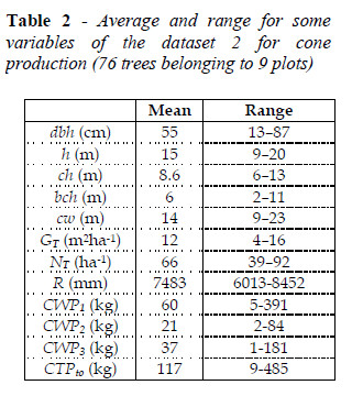
For dataset 1 the dependent variable in the modelling is the global cone weight production per tree for the three production periods. For dataset 2 the dependent variable is the cone weight production per tree for each production period. Tree and plot covariables were used as independent variables. The two kinds of models can integrate intercept, slope, and nested random effects.

In Tables 1 and 2 the variables CWP₁, CWP₂, CWP₃ and CWP_to correspond to the average production per tree of the global production for each of the three production periods (1:2004-2005, 2: 2004-2005 and 3:2004-2005). The variable CWP_to corresponds to the average production per tree in the three periods. Data from local automatic weather stations (Portuguese Meteorological Institute), available online (http://snirh.apambiente.pt) allowed computing accumulated rainfall (AR) for five-year periods precedent to each of the three production periods.

The average cone production per tree in the dataset 1 was 61 kg, respectively. The average N_T was 89 trees ha^-1. The higher tree cone yield (over 200 kg/tree) was shown in bigger trees (dbh greater than 60 cm, cw above 12 m and h above 14 m). The higher cone production (in the range 3000 - 7000 kg ha^-1)occurred in stone pine plots with a G_T of 5 - 21 m² ha^-1and 40 - 176 trees ha^-1.

A logarithmic transformation (natural log) of cone weight production per tree allowed obtaining a Gaussian distribution (graph not shown) for the transformed data, more appropriate to fit linear (Gaussian) mixed models. Table 3 shows the sample correlation matrix of these data revealing that, as expected, some independent variables are strongly correlated, with correlation measures greater than 0.7, reflecting multicollinearity between variables. These high correlations implicate a selection of the independent variables to fit with the linear mixed models for quantifying cone production.

The higher correlations, highlighted in Table 3, are: i) h with both HD and bch (0.81 and 0.77, respectively), ii) c with both g and CA (0.86 and 0.99, respectively), iii) Dh with G_T, G_SP and bch (0.87, 0.83 and 0.70, respectively), iv) N with N_T (0.91), v) G_Twith both G_SP and bch (0.98 and 0.72, respectively, vi) g with Ca (0.86), vii) G_SP with bch (0.73).

For the modelling of cone production with the dataset 1 (Table 1), we firstly made a screening analysis of independent biometrical variables, by least squares regression of two ensembles of 13 and 7 covariables and of 14 ensembles of four, three, two and one covariables for detecting the ensembles of independent covariables with lower collinearity (low variance inflation factor), and higher coefficient of determination between them. Table 4 displays collinearity and AIC statistics for the 14 ensembles of independent variables. The two ensembles with higher number of variables showed, as expected, high level of collinearity between covariables and were discarded for posterior analysis. To a subsequent selection, the 14 ensembles of variables were submitted to a LMM fitting process, under a two level clustered data structure, with an intercept term, using the SAS PROC MIXED (Version 9.1.3). This selection was based on the information criteria (-2log likelihood and AIC) and the fixed and random parameters significance and on a general residual diagnostic (INFLUENCE option of PROC MIXED) as well.

Modelling

Classic linear mixed models

For modelling cone production per tree with the first dataset we used classic LMMs. The methodology was the restricted maximum likelihood estimation (REML), summarized below (eqs. 1-10), implemented in SAS Proc MIXED (Version 9.1.3). LMMs, relying on asymptotic normality, are attractive due to their ability to deal with multiple levels of data clustering. As mentioned above, LMMs have become invaluable tools in the analysis of experimental and observational data of hierarchical, clustered, longitudinal or spatial kinds, allowing for more than one term to be submitted to random variation.

The general matrix equation for LMMs (SEARLE, 1971) can be written as:

where y_i represents the continuous response vector of n_i known observations (trees) for the i-th sampling unit (plot), X_i is the ( n_i x p) design matrix of known elements of observations related to p independent variables or covariables, ß is the unknown vector of p regression coefficients (fixed effect parameters), Z_i is a ( n_i x q) design matrix associated to random effects, whose terms may be ones, zeros or measured values for the q predictor variables for the i-th plot, u_i is a vector of q random effects and e_i is a vector of n_i residuals for the i-th sampling unit. The number of observations for each plot, n_i, is not necessarily equal, i = 1,...,51.

Random vectors u_i and e_i are assumed to have multivariate normal distribution:

where 0 is a null vector, D is the (qxq ) symmetric positive-definite variance-covariance matrix of random effects, and R_i is the ( n_iXn_i) symmetric positive-definite variance-covariance matrix for the residual matrix in the i-th subject (plot).

The REML estimation is based on an iterative optimization of the so called REML log-likelihood function (e.g., WEST et al., 2007):

with:

where is the total number of observations, is the vector of all model parameters and V_i is the n_ixn_i matrix corresponding to the implied marginal or population-averaged model for subject i:

where the marginal residual vector is y_i ~ N(0, V_i), and the estimated form of variance-covariance matrix V_i ( n_ixn_i) is given by:

After obtaining an estimation of V_i, the following equations are used to estimate the fixed effects parameters and their standard errors:

In this work, for dataset 1, a LMM was fitted considering the two-level hierarchy for independent variables, plot and tree, and the variance components and identity structures for covariance matrices for random effects and residuals, respectively.

The two criteria for model selection are the so-called information criteria that are mainly i) the –2 res log-likelihood criterion, , ii) the Akaike information criterion (AIC) (AKAIKE, 1974):

where l is the log-likelihood function, which is evaluated at the REML estimates of the model parameter vector ( ), and p is the total number of parameters, including the fixed and random effects. The best model is that for which calculations of the criteria give the smaller values. This methodology allows comparing any models fitted to the same data whether they are nested or not. The estimation of the random effects is given by the empirical best linear unbiased predictors, u_i (EBLUPS), (SEARLE, 1971):

Residual diagnostics in linear mixed models

Influence diagnostics of a fitted LMM allows verifying whether the distributional assumptions for the residuals are valid and whether the fitted model is sensitive to individual observations. The basic approach of this diagnostics methodology is to quantify the effects of an omission of a given subset of observations, in our case a plot (cluster unit), denoted by a subscript, U,on the global results of the analysis of the entire data. The model is refitted and statistics are computed based on the change between full data and reduced data estimation. The INFLUENCE option in SAS Proc Mixed (Version 9.1.3) allows the calculation of statistics for this kind of analysis and also the generation of panels of influence. This approach is similar to residual analysis applied to ordinary least squares analysis (e.g., NETER et al., 1996).

In this work, we used data and panels of unconditional and conditional studentized residuals, restricted likelihood distance, PRESS residuals, Cook's D, covratios, covtraces and MDFITTS for fixed and random effects.

Basically, unconditional and conditional residuals are defined respectively as:

The residual studentization diminishes the impact of one problem of the raw residual, variance heterogeneity. The studentized form of these raw residuals is given by a scaling of the form (LITTELL et al., 2007):

where an estimate of the variance of the residuals is placed in the denominator and h_ii is the i-th diagonal element of the leverage matrix (H):

The restricted likelihood distance (RLD) is given by:

where l_R is the restricted likelihood function, and is an arbitrarily chosen vector of parameters, which can include parameters in ß or . RLD reflects the change in REML log likelihood for all data, with estimated for all data, , and reduced data, (u). To the definitions of PRESS residuals, Cook's D, covratios, covtraces and MDFITTS for fixed and random effects, refer to LITTELL et al., 2007.

Bayesian clustered longitudinal mixed models

For the second dataset, with cone production data available for the three production periods, three longitudinal models were fitted from a Bayesian perspective. Basically, the Bayesian analysis is based on a scaled product of a likelihood function L(D|), dependent on the available data D and the model parameter vector , by the prior distribution for , p(), representing the probability that takes any particular value based on prior information available. The result is the posterior distribution for , p(|D), expressing what is known about given the sample data.

For smaller sample sizes, Bayesian inference is especially advantageous over likelihood-based inference because the latter is related to asymptotic theory. Thus, Bayesian analysis can provide more reliable information than classic theory for LMMs, namely estimating the variance component of the random effects (PAULINO et al., 2003, and GELMAN et al., 2006).

The Bayesian clustered longitudinal mixed models, considered for the second dataset, were fitted taking on account random effects for clustered data with three levels of hierarchy: plot as level 3, tree as level 2, and production period (for simplification designated as time) as level 1 (Figure 1). The difference between these models and the previous ones consisted in the incorporation of two additional random effect vectors, associated with trees (sampling units) nested within a plot (cluster), Eq. 16, and with plots sharing time slope random effects. Therefore, the longitudinal clustered mixed models are expressed as:

 

 

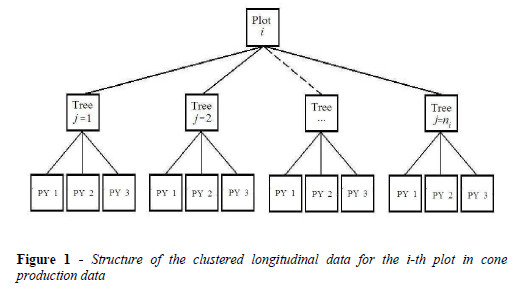
where y_ti represents the response vector of n_i observations (trees) for the i-th sampling unit (plot) at the th-production campaign, X_ti is the design matrix related to p possibly time-dependent covariables, u_0i and u_1i are random (plot) effect vectors associated with the intercept and time slope, respectively, u_2(i)is the random effect vector associated with trees nested within a plot, and e_ti is a vector of n_i residuals for the i-th sampling unit at the th-production campaign, i =1,...,9 , t =1,...,3. The nested plot effects correspond to random effects associated to the plots, reflecting environmental or genetic variables not measured in our experimental design. Notice that, i) the random effects, u_0i and u_1i, were representative of variability inherent to the plot and to the production period, respectively, and ii) two sub-models from Eq. 16 are designed hereafter as (16*) and (16**) after removing the time slope (u_1i) and nested (u_2(i)) random effects and only the nested (u_2(i)) random effects, respectively.

In this work, random vectors u_0i, u_1i and u_2(i), and e_ti are assumed as multivariate normally distributed:

where D₀, D₁, and D₂ are the (q x q) symmetric positive-definite covariance matrix of the random effects u_0i, u_1i and u_2(i), respectively, and R_ti is the symmetric positive-definite covariance matrix (n_i x n_i) for the residual matrix in the i-th subject (plot) at time point i, (i = 1, …, 9, t = 1, 2, 3). These covariance matrices were considered:

where I is the identity matrix, proportional to the appropriate Gaussian likelihood function times associated with prior distribution. We assumed also (independent) normal prior distributions for regression coefficients ß with mean zero and variance v²_k (known), k=0,…,p (number of independent variables), and independent inverse gamma prior distributions for the variance components:

Consequently, the joint posterior distribution of for longitudinal mixed model in Eq. 16 is expressed by

where and (response mean).

The posterior in Eq. 20 is awkward to work with, since the marginal posterior distributions of are not easy to obtain explicitly. Numerical methods can be employed in order to overcome that problem, e.g., Markov chain Monte Carlo (MCMC) methods that are implemented in software such as OpenBugs (LUNN et al., 2009). MCMC simulation involves simulating a sample from the joint posterior distribution of the model parameters using one of three main algorithms: Metropolis Hastings, Gibbs sampling and slice sampling. It is thereby possible to generate numerically, with a sufficient large sample, the posterior distribution from which inferences of interest can be made. For example, ZEGER and KARIN (1991) coped with generalized linear models under a Bayesian framework using the Gibbs sampler to solve computational limitations, whereas FONG et al. (2010), confirmed the appealing Bayesian approach for LMMs by implementing prior distributions with variance components by the use of integrated nested Laplace approximations.

For the adequacy of fitness diagnostics of the Bayesian models, we used three criteria: i) the posterior mean of the deviance (-2 log-likelihood function), ii) the deviance information criterion (DIC), which is a generalization of AIC, proposed by SPIEGELHALTER et al. (2002) and calculated as:

where PD is the effective number of the model parameters (a smaller DIC indicates a better model fitness), and iii) the conditional predictive ordinate (CPO, GELMAN et al., 2004), defined by the posterior predictive distribution:

where y_i is the observation i of the data y, and y_[i] is y without the current observation i, being p(y_i|) a predictive distribution and p(|y_[i]) a joint posterior distribution for the model parameter . The CPO is based on the leave-one-out cross-validation predictive density, and is easy to obtain with MCMC methods. It may be used to identify outliers, influential observations, and for hypothesis testing across different non-nested models.

 

Results and discussion

Cone production by LMMs

The selected two level clustered LMM model with an interception term (cone weight production by tree) was the following:

where lnCWP_ijis the natural logarithm of the weight cone total production of the j_thtree belonging to the i_thplot (i=1,...,51) and the other tree and plot variables correspond to crown width, basal area by hectare and tree height, respectively. The terms u_iand e_ij correspond respectively to random intercepts, specific to each plot, and residuals, defined above (Section 2.2.1). The estimated parameters for this model [Eq. 23] are shown in Table 5.

 

 

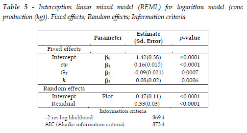
The selected LMM [Eq. 23] showed that two tree variables, the crown width (cw_ij) and the tree height (h_ij), and a plot variable, the total basal area by hectare (G_Ti), were highly influential variables to predict cone production. The dependent variables cw_ij and G_Ti are easy to obtain. Measurement of tree height, a variable associated to site index, is not so practical, leading to the need of modelling height-diameter relationship.

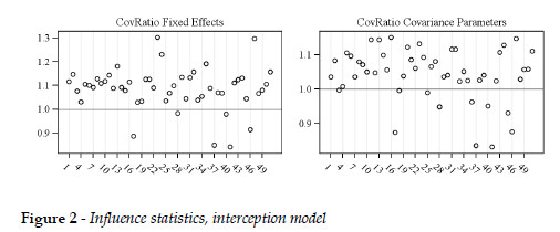
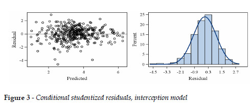
The average influence residual statistics for the selected LMM are shown in Table 6. These statistics are in reasonable agreement with reference values of zero for Cook'D, MDFFITS and Covtrace and PRESS residuals, and of one for Covratio. The restricted likelihood distance, with the average value of 0.25 and a standard deviation (Table 6) of 0.009 fits well with a reference value, corresponding to the 75th percentile for a chi-square distribution with six degrees of freedom (total number of fixed and random parameters in the interception model) of about 10. This means that the log likelihood estimation of the full data is not affected by data sampling reduction (WEST et al., 2007). Figure 2 depicts Covratio statistics for fixed effects and covariance parameters. Although the PRESS statistic shows deviation from zero, its graphical display (not shown) is in reasonable agreement with some references (e.g., WEST et al., 2007; LITTELL et al., 2007). Conditional studentized residuals (Table 6 and Figure 3), follow the typical Gaussian distribution.

 

 

 

 

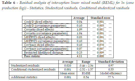
The positive values of ß₁ (associated to c) and ß₃ (associated to h) and the negative ß₂ (associated to G_T) are indicative that in general terms, bigger trees with larger crowns and lower plot density and competition are the ones with greater cone production. This coincides with conclusions in previous works (e.g., CAÑADAS, 2000; ALPUÍM et al., 2000; CALAMA, 2004, CALAMA et al., 2008; FREIRE, 2009). ALPUÍM et al. (2000), for Portuguese stone pine stands, noted that under similar ecological conditions stone pine fructification depends mainly on the crown diameter.

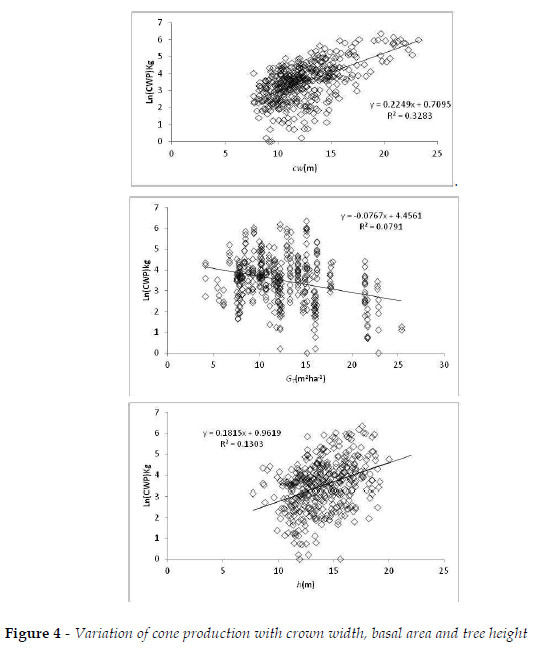
The selected model (Eq. 23), reflected the cone production variability by single least squares regression with its dependent variables (Figure 4). Indeed, the more productive plots were originated from natural regeneration, managed to cone production since the beginning of productive cycle, with thinning operations to low tree densities, irregular distribution, allowing for crown development and diameter at breast height enlarging with the canopy area covering about 53 % to 73 % of forest surface. Plot randomness explained 58% of global variability (Eq. 25) and therefore the inclusion of random effects associated with plots, allowed to improve the quality of estimates. Given that the experimental plots were located in the same productive region (Setúbal Peninsula), thus minimizing regional effects, we think that factors such as distinct productive stages, environmental site conditions, distinct topography, allowing for water accumulation by gravity, same genetic variation due to predominant natural regeneration, and also the drought anomaly in 2004/2005 (RODRIGUES et al., 2011) explained most of the global heterogeneity in cone production. The precipitation accumulated in five-year periods, prior to each of the three production periods, evidenced no significant effect on global cone production, circumstance due, from our point of view, to the fact that the global dataset included all data irrespective of the production year. Eq. 23 can be used to obtain estimates of plot specific cone production in a three-year period, using the calculated EBLUPS per plot. The same equation can be used to obtain population-averaged production in the same period to all productive area, by omitting random effects.

 

 

Cone production by Bayesian clustered longitudinal analysis

For the second dataset (Table 2) related to three production periods, several Bayesian linear mixed models [in Eq. (16), including (16*) and (16**)] were fitted assuming flat prior distribution [Eq. (17)- (19)] with , a = ak = b = bk = 0.001 , k=0,1,2, v₂j =10₆ , j=0,1,…p, since such values avoid an excess of information for a non-informative setting. Besides, the results of this Bayesian analysis were obtained through the software OpenBugs (LUNN et al., 2009) after 50000 iterations of simulation and 2000 iterations of burn-in.

Table 7 displays a model comparison based on DIC and Deviance posterior mean for clustered longitudinal data. The second column in Table 7 is related to no-time slope and no-nested clustered longitudinal model (16*), whereas the third column reports no-nested clustered longitudinal model (16**). In the last two columns are indeed the fitting results of the comprehensive three-level clustered longitudinal models [Eq. (16)]. In that table, there are the better fitting longitudinal mixed models, i.e., models M₁,M₂,M₃ andM₄ that were defined from sets of the covariables: dbh, h, cw,HD, DD, N, G_T, g,CA, G_SP, N_T, bch, ch, time (production period) and AR. DIC and Deviance values indicate that linear model in Eq. (16) is better fitted, and the former values point out in favour of M₃ for both model comparison measures. Notice that DIC takes into account the complexity of the model, which is an important issue in mixed models, and the selected model M₃ [Eq. (16)] has better fitting even than parsimonious model M₄.

 

 

The selected model, representative of average annual production in the t-th campaign (time) of the j-th tree belonging to the i-thplot, (i = 1, …, 9, j=1,…, 76, t = 1, 2, 3) is expressed by

where lnCWP_tijis the natural logarithm of the weight cone production for tree j in plot i at production period t, and the other variables correspond to crown width (cw_ij), five -year accumulated rainfall (AR_t), time t (for convenience, assuming values -1, 0 and 1), and u_0i, u_1i, and u_2(i)j are the random intercept, time slope and nested (plot) effects, and e_tij is the residual term, i=1,…, 9, j=1,…, 76, t=1,2,3. This model also showed the complexity of the cone production process, by including random factors associated to the production period, related to the variability between production years, and nested plot effects, related to the local variables of stand, environmental or genetic type associated to the plots themselves, not measured under our experimental design. Posterior estimates based on the selected clustered longitudinal model [Eq. (24)] are shown in Table 8: posterior mean, standard deviation (s.d.), median and 95% credible interval of some random parameters of interest. The selected covariables, crown width (cw_ij) and five-year accumulated rainfall (AR_i), have a positive influence on the weight cone production, indicating that a greater discrepancy in cw_ij and AR_i is associated with a higher mean value of lnCWP_tij. The variable cw_ij is common to the two selected models in Eq. (23) and Eq. (24), with a coefficient of the same order of magnitude, reflecting the relevance of crown width in cone production. The rainfall was relevant on longitudinal data of cone production per production period, reflecting the fact that globally, weight cone production in all plots encompassed by this study, was higher in 2004/05 (4578 kg), decreasing substantially in 2005/06 (1601.8 kg), and recovering partially in 2006/07 (2821 kg). The reduction in 2005/06 may reflect the aforementioned drastic diminution in rainfall occurred in the period 2004/05.

 

 

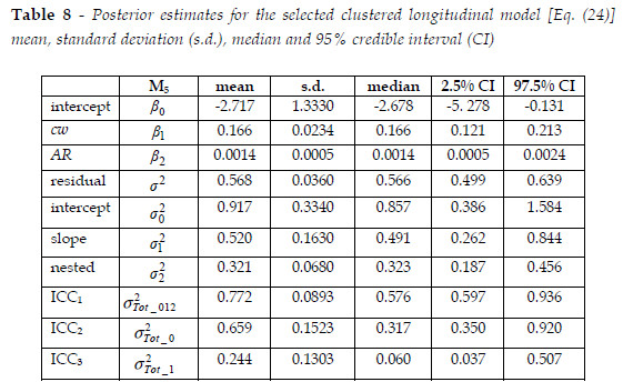
In Table 8 variance component estimates were obtained for the selected model [Eq. (31)]. These include the variance of the intercept (), time slope ( ) and nested () random effects, apart from the variance of the residual terms (). There is some unobserved heterogeneity at the three levels of data in decreasing order (Table 8) by overall plot effect (0.917), time plot effect (0.52) and individual tree within plots effect (0.321), and some residual heterogeneity among trees (0.568). The intraclass correlation coefficient (ICC) (WEST et al., 2007) is calculated from the several estimated "total" variance components as follows:

Thereby it can be inferred that most of the total variation in the weight cone production per tree is dominated by the random plot effects (0.772), comparing with 0.7 from LMM in Eq. (23), and this random variation is due to overall among-plot (65.9%) and time slope among-plot (24.4%) effects.

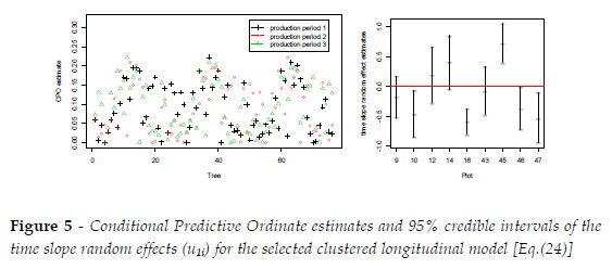
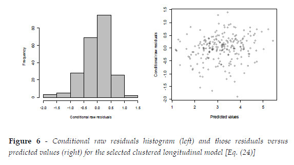
For assessment of mixed model in Eq. (24), CPO [Eq. (22)] estimates were plotted in Figure 5 (left side), ranging from 0.000001 to 0.2215, depicting no outliers and influential values for all three production periods. In addition, conditional raw residuals, Eq. (11), were obtained and plotted in Figure 6 suggesting no specific model fitting problem both from its histogram (left side) and from its comparison with corresponding predictive values (right side). In Figure 5 (right side) there is a graphical representation of time slope random effect estimates and 95% credible intervals pointing out that plots 10, 16, 45, 46, and 47 have significant random effects over time. In these plots, an average N_T of 91 ha^-1, above a global average of 66 ha^-1, indicates an occupation of mainly younger trees, and thereby the occurrence of significant time random effects reflects a higher longitudinal variability in younger stands.

 

 

 

On the other hand, Eq. (24) includes nested plot effects, associated to the plots, not measured and probably associated to micro-environmental and genetic factors, reflecting their relevance to the cone production process

 

Conclusions

This work aimed to develop linear mixed models under classic and Bayesian approaches for cone pine production in the Portuguese Setúbal Peninsula, based on cone weight production data in stone pine plots during three production periods. The two-level clustered linear model was estimated from all cone production data available for three consecutive years, including plots from which the production data collection was not possible for every year of the period considered. This model included crown width, total basal area per hectare and tree height as dependent variables determinant for cone production. The Bayesian three-level clustered longitudinal linear model was obtained from a data subset, referring to plots from which production data collection was possible in all the three productive periods. In this model, crown width and five-year accumulated rainfall, prior to each production period were included as the independent variables determinant for cone production. The complexity of the cone production process in the field was reflected by the inclusion in the Bayesian equations of random factors associated to the production period, and to nested plot effects, related to the local environmental or genetic variables of the plots. These variables should be considered under a throughout experimental design. The variables selected for both models agree with results from other studies on stone pine cone production. In both models the intra-cluster variance, expressing the randomness associated to plot effects, significantly contributes to more than 58% of the global variability and thereby justifies an experimental design based on data clustering in plots and production years.

With a dataset limited to only three production periods, the aimed objectives had only a preliminary significance, given the fact that long term empirical evidence suggested that cone production follows a 7–8 year campaign cycle. Despite the small period of data collection the results obtained are indicative about the tree and stand variables adequate for proper forest management aiming at cone production. The results obtained are still conjectural for the Portuguese stone pine forest, and an extension both of measurement period and other productive zones are obviously needed for a more thorough and representative analysis.

 

References

AKAIKE, H., 1974. A new look at the statistical model identification. IEEE Transactions on Automatic Control 19(6): 716–723.         [ Links ]

ALPUÍM, M., BAETA, J., CARNEIRO, M.M., CARVALHO, M.A., ROCA, M.E., PESSOA, J., 2000. Classification of stone pine selected for pine kernels production, IUFRO International Meeting. May, Sevilla, Spain.         [ Links ]

CALAMA, R., 2004. Modelo Interregional de Silvicultura para Pinus pinea L. Aproximación mediante funciones con componentes aleatorios. Tesis Doctoral, Escola Técnica Superior de Ingenieros de Montes, Universidade Politécnica de Madrid 307pp.         [ Links ]

CALAMA, R., MONTERO, G., 2005. Cone and seed production from stone pine (Pinus pinea L.) stands in Central Range (Spain). Eur. J. Forest Res. 126(1): 23–35.         [ Links ]

CALAMA, R., MONTERO, G., 2006. Stand and three-level variability on stem form and tree volume in Pinus pinea L.: a multilevel random components approach. Invest. Agrar: Sist. Recur. For. 15(1), 24–41.         [ Links ]

CALAMA, R., MADRIGAL, G., CANDELA, J.A., MONTERO, G., 2007. Effects of fertilization on the production of an edible forest fruit: stone pine (Pinus pinea L.) nuts in south-west Andalusia. Invest. Agrar: Sist. Recur. For. 16(3): 1–12.         [ Links ]

CALAMA, R., GORDO, F.J., MUTKE, S., MONTERO, G., 2008. An empirical ecological-type model for predicting stone pine (Pinus pinea L.) cone production in the Northern Plateau (Spain). Forest Ecology and Management 255: 660–673.         [ Links ]

CAÑADAS, M.N.C., 2000. Pinus pinea L. en el Sistema Central (valles del Tiétar y del Alberche): desarrollo de un modelo de crecimiento y producción de piña. Ph. Dr. Thesis. Universidad Politécnica de Madrid, 356pp.         [ Links ]

CARRASQUINHO, I., FREIRE, J., RODRIGUES, A., TOMÉ, M., 2010. Selection of Pinus pinea L. plus tree candidates for cone production. Ann. For. Sci. 67: 814. DOI:10.1051/forest /2010050.         [ Links ]

FONG, Y., RUE, H., WAKEFIELD, J., 2010. Bayesian inference for generalized linear mixed models. Biostatistics 11(3): 397–412.         [ Links ]

FREIRE, J., 2009. Modelação do crescimento e da produção de pinha no pinheiro-manso. PhD Thesis, Instituto Superior de Agronomia, Universidade Técnica de Lisboa.         [ Links ]

GELMAN, A., CARLIN, J., STERN, H., RUBIN, D., 2004. Bayesian Data Analysis. 2^nd edition. Chapman & Hall, Boca Raton, FL.         [ Links ]

GONÇALVES, A.C., POMMERENING, A., 2012. Spatial dynamics of cone production in Mediterranean climates: A case study of Pinus pinea L. in Portugal. Forest Ecology and Management 266: 83–93.         [ Links ]

GARCÍA GÜEMES, C., 1999. Modelo de simulación silvicola para Pinus pinea L. en la província de Vallalodid. PhD Thesis. Escuela Técnica Superior de Ingenieros e Montes. UPM. Madrid.         [ Links ]

ICNF, 2013. Inventário Florestal Nacional (Portugal Continental) Lisboa. http://www.icnf.pt/portal/florestas/ifn/ifn6.         [ Links ]

KOENIG, W.D., KNOPS, J.M.H., CARMEN, W.J., STANBACK, M.T., MUMME, R.L., 1996. Acorn production by oaks in central California: influence of weather at three levels. Can. J. For. Res. 26: 1677–1683.         [ Links ]

LITTELL, C.R., MILLIKEN, G.A., STROUP, W.W.; WOLFINGER, D.W., SCABENBERGER, O., 2007. SAS for Mixed Models. Second Edition. SAS Institute Inc., 813pp.         [ Links ]

LUNN, D., SPIEGELHALTER, D., THOMAS, A., BEST, N., 2009. The BUGS project: Evolution, critique, and future directions. Statistics in Medicine 28: 3049–3067. OpenBugs version 3.2.1, 2011: http://www.openbugs.info/w/.         [ Links ]

MUTKE, S., GORDO, F.J., GIL, L., 2000. Seleccion de indivíduos de Pinus pinea L. grandes productores de fruto en las masas de la meseta norte. In: 1^er. Simposio del pino pinonero (Pinus pinea L.). 22- 24 de February 2000, Valladollid. Edited by Junta de Castilla Y León Tomo II, 85–93.         [ Links ]

MUTKE, S., GORDO, F.J., GIL, L., 2005. Variability of Mediterranean stone pine cone production: yield loss as response to climatic change. Agric. For. Met. 132: 263–272.         [ Links ]

NETER, J., KUTNER, M.H., NACHTSHEIM, C.J., WASSERMAN, W., 1996. Applied linear statistical models,. WCB/McGraw Hill, 1408pp.         [ Links ]

PAULINO, C.D., AMARAL TURKMAN, A., MURTEIRA, B., 2003. Estatística Bayesiana. Fundação Calouste Gulbenkian, Lisbon, 446 pp.         [ Links ]

SEARLE, S.R., 1971. Linear Models. John Wiley & Sons, 532 pp.         [ Links ]

SEARLE, S.R., CASELLA, G., MCCULLOCH, 2006, Variance components. John Wiley & Sons, 501 pp.         [ Links ]

SPIEGELHALTER, D.J., BEST, N.G., CARLIN, B.P., VAN DER LINDE, A., 2002. Bayesian measures of model complexity and fit (with discussion). Journal of the Royal Statistical Society B 64(4): 583–639.         [ Links ]

SUROVÝ, P, RIBEIRO, N., PEREIRA, J.S., 2011. Observations on 3-dimensional crown growth of stone pine. Agroforestry Systems 82: 105-110.         [ Links ]

WEST, B.T., WELCH, K.B., GALECKI A.T., 2007. Linear mixed models. A practical guide using statistical software. Taylor and Francis Group, 353pp.         [ Links ]

ZEGER, S.L, KARIN, M.R., 1991. Generalized linear models with random effects: a Gibbs sampling approach. J. Amer. Statist. Assoc. 86: 79-86.         [ Links ]

 

Submitted for publication in May 2014

Accepted in June 2014

 

Acknowledgements

This study was supported by the AGRO 451 project "Stone Pine Stand Improved and Management Optimization for Cone and Seed Production". Giovani L. Silva was partially supported by Pest-OE/MAT/UI0006/2011.