


 Inglês (pdf)
 Artigo em XML
 Referências do artigo
 Enviar este artigo por email
 Citado por SciELO
  Similares em
SciELO
Similares em
SciELO 
 Permalink
Introduction
As a direct result of industrialization and technical advancement, more than 90% of current construction equipment is made of CS 1. CS is used in chemical processing, oil drilling and refining, pipelines, mining, construction and metal-processing equipment, despite its low corrosion resistance 2-4. It is widely used due to its high strength, durability and cost-effectiveness 5-8. Welding is a common method of joining different sections of CS pipes, structures and equipment, in manufacturing, marine, oil and gas industries 9-10.
However, CS welding in industrial application requires stringent procedures, to ensure safety and structural integrity 11. When exposed to aggressive media commonly found in Sw media, CS is vulnerable to corrosion 12-14. Corrosion of CS welds in Sw is a common problem, due to the aggressive nature of this environment. The presence of chloride ions, high salinity and dissolved oxygen accelerates the corrosion process, leading to a weakened weld that can fail prematurely 15,16. Therefore, proper surface preparation, PWHT, coating, inspection and routine maintenance are essential to prevent corrosion and ensure long-term structural integrity 17,18.
RSM is a statistical and experimental design method that uses a selected dependent variable and deviations in one or more independent or factor variants 19-24. This technique helps to predict corrosion properties, if it is effectively modelled and optimized, as reported in literature 26,39,40. RSM is used to determine the optimal value for dependent variables, by adjusting design parameters for the independent ones 27. Using a range of experimental design software applications and methodologies, corrosion prediction models have been developed 28-31. GC analysis, a basic and cost-effective analytical method 32,33, can be used to determine WL and CR of metals and alloys exposed to aggressive media. After establishing the mass loss over time, this evaluation method may be employed to predict CR of the material in actual service. This work strived for identifying optimal CP and models for an effective corrosion study of welded CS exposed to a Sw environment, using RSM approach.
Experimental methods
Data collection
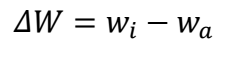
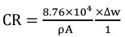
For this design optimization and modelling investigation, experiment data obtained from a corrosion study using GT were employed. The effectiveness of post-weld tempering (at 25, 550, 650 and 700 ºC) in protecting CS welds from corrosion in a Sw environment was evaluated. As-welded and PWT samples (550, 650 and 700 ºC) were weighed and completely immersed by suspension in a Sw test media contained in plastic containers, for different ET of 17, 34, 51, 68 and 85 days. The samples were taken out after a specific ET was reached. Corrosion products were removed by washing the samples with distilled water, in acetone, and drying them in ambient air. The coupons were then reweighed, to determine their final weights. Experimental data were collected and analyzed using Eqs. 1 and 2.
 ()1
()1
 ()2
()2
where ∆W is change in mass (g), Wi and Wa represent the coupon’s initial and final weights, respectively, ρ is density (7.85 g/cm3), A is the exposed surface area in cm2 and t is time in h.
CCD
According to GT results, post-weld tempering and ET had a significant impact on WL and CR of CS. A two-factor, two-level CCD 34 was used to compare the effects of post-weld tempering and ET on WL and CR of the alloy. Table 1 shows the levels of the independent variables used for constructing experiments to determine corrosion properties. By conducting the experiments at random, errors were minimized. 20 runs were generated by the design matrix. Data statistical analysis was performed using Design Expert 11. Research works reported by 35-37 describe the fundamental steps of the optimization procedure, which include: conducting the statistical design experiments; determining the coefficient in a mathematical model; predicting the response and confirming the model adequacy, as set up in the experiment; and validating the predicting model.
Results and discussion
RSM results
RSM results are presented in Table 2. The interactive effects of post-weld tempering T and ET on WL and CR are shown based on the considered factors. These results suggest that the relationship between WL and CR decreased with increased post-weld tempering T and ET.
Table 2: RSM variables predicted responses data.
| Factor 1 | Factor 2 | Response 1 | Response 2 | ||
|---|---|---|---|---|---|
| SD | Run | A: T of PWT (oC) | B: ET (days) | WL (g) | CR (mm/yr) |
| 15 | 1 | 650 | 85 | 0.0282 | 0.0245 |
| 11 | 2 | 25 | 34 | 0.7208 | 0.5489 |
| 13 | 3 | 650 | 51 | 0.298 | 0.1029 |
| 12 | 4 | 650 | 34 | 0.2901 | 0.1708 |
| 6 | 5 | 550 | 17 | 0.3321 | 0.3739 |
| 3 | 6 | 25 | 51 | 0.6829 | 0.3483 |
| 19 | 7 | 700 | 68 | 0.1508 | 0.0231 |
| 4 | 8 | 25 | 68 | 0.5098 | 0.1669 |
| 2 | 9 | 550 | 68 | 0.3145 | 0.1064 |
| 14 | 10 | 550 | 85 | 0.1183 | 0.0556 |
| 10 | 11 | 650 | 17 | 0.1871 | 0.2579 |
| 9 | 12 | 700 | 17 | 0.1066 | 0.195 |
| 8 | 13 | 550 | 51 | 0.4156 | 0.1764 |
| 20 | 14 | 700 | 85 | 0.0248 | 0.004 |
| 5 | 15 | 650 | 68 | 0.2107 | 0.0541 |
| 7 | 16 | 700 | 34 | 0.2165 | 0.1185 |
| 16 | 17 | 650 | 85 | 0.0282 | 0.0245 |
| 18 | 18 | 25 | 85 | 0.2416 | 0.0046 |
| 17 | 19 | 550 | 34 | 0.4214 | 0.2656 |
| 1 | 20 | 25 | 17 | 0.7435 | 0.7686 |
ANOVA for WL and CR
Statistical ANOVA is presented in Tables 3 and 4, respectively, which show the model’s F-values of 18.34 and 77.38, for WL and CR of CS, respectively. Results also indicate that the probability of an elevated F-value due to the system SNR is less than 0.01%. Microstructural modifications in CS samples caused by welding may account for variations 33. The probabilities of failure (prob > F) with values lower than 0.050 for both variables are shown in Tables 3 and 4. This outcome implies that A, B, AB, A2 and B2 generated model terms are significant.
Predicted R2 values for WL (0.8676) and CR (0.9651) exhibit significant agreement with their corresponding adjusted R2 (0.8203 and 0.9526, respectively). The variation below 0.2 of R2 indicates a high level of statistical agreement between actual and predicted values. The adequacy of precision was determined by evaluating SNR, which is seen as entirely acceptable, if higher than 4. Since WL and CR obtained a SNR of 14.2119 and 32.117, this strongly indicates the model’s good performance, and its ability to effectively navigate the design space. Hence, it can be concluded that the quadratic regression model was effective in predicting WL and CR of CS, both in its as-welded and PWT states, when exposed to a Sw environment 33. A polynomial quadratic regression model was created to establish the relationship between WL and CR of CS, which are shown in Eqs. 3 and 4.
 ()3
()3
 ()4
()4
Table 3: Quadratic ANOVA model for WL of UNS G10400 CS.
| Source | Sum of squares | DFF | Mean square | F-value | p-value | |
|---|---|---|---|---|---|---|
| Model | 0.9342 | 5 | 0.1868 | 18.34 | < 0.0001 | significant |
| T of A-PWT | 0.5858 | 1 | 0.5858 | 57.52 | < 0.0001 | |
| ET of B | 0.2098 | 1 | 0.2098 | 20.6 | 0.0005 | |
| AB | 0.0545 | 1 | 0.0545 | 5.35 | 0.0365 | |
| A² | 0.0214 | 1 | 0.0214 | 2.1 | 0.1696 | |
| B² | 0.1268 | 1 | 0.1268 | 12.45 | 0.0033 | |
| Residual | 0.1426 | 14 | 0.0102 | |||
| Total corr. | 1.08 | 19 | ||||
| SD | 0.1009 | R² | 0.8676 | |||
| Mean | 0.3118 | Adj. R² | 0.8203 | |||
| CV% | 32.37 | Pred. R² | 0.6888 | |||
| Adeq. precis. | 14.2119 |
| Source | Sum of squares | DF | Mean square | F-value | p-value | |
|---|---|---|---|---|---|---|
| Model | 0.731 | 5 | 0.1462 | 77.38 | < 0.0001 | significant |
| T of A-PWT | 0.2367 | 1 | 0.2367 | 125.3 | < 0.0001 | |
| ET of B | 0.477 | 1 | 0.477 | 252.49 | < 0.0001 | |
| AB | 0.1303 | 1 | 0.1303 | 68.97 | < 0.0001 | |
| A² | 0.008 | 1 | 0.008 | 4.24 | 0.0586 | |
| B² | 0.0051 | 1 | 0.0051 | 2.71 | 0.1217 | |
| Residual | 0.0264 | 14 | 0.0019 | |||
| Total corr. | 0.7574 | 19 | ||||
| SD | 0.0435 | R² | 0.9651 | |||
| Mean | 0.1914 | Adj. R² | 0.9526 | |||
| CV% | 22.71 | Pred. R² | 0.8825 | |||
| Adeq. precis. | 32.117 |
Interactive analysis of CS
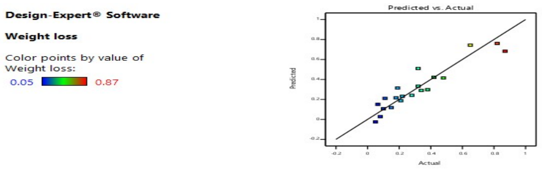
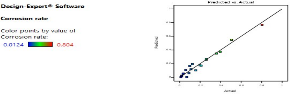
Figs. 1, 2, 3 and 4 illustrate graphical representations of WL and CR pertaining to the vulnerability of welded and tempered CS samples in a Sw medium. The plots depicted in Figs. 1 and 2 exhibit a linear relationship between predicted and actual WL and CR. The data points exhibited a tendency to cluster in close proximity to the best fit line. The results indicate that the chosen quadratic model was suitable for predicting WL and CR of CS in a marine environment.
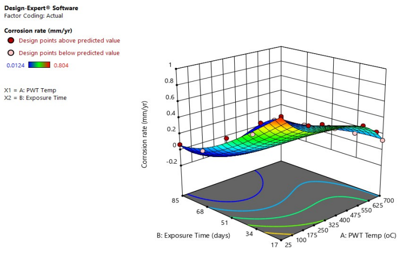
Figs. 3 and 4 depict 3-D graphical representations of interactive effects resulting from the combination of post-weld tempering and ET.
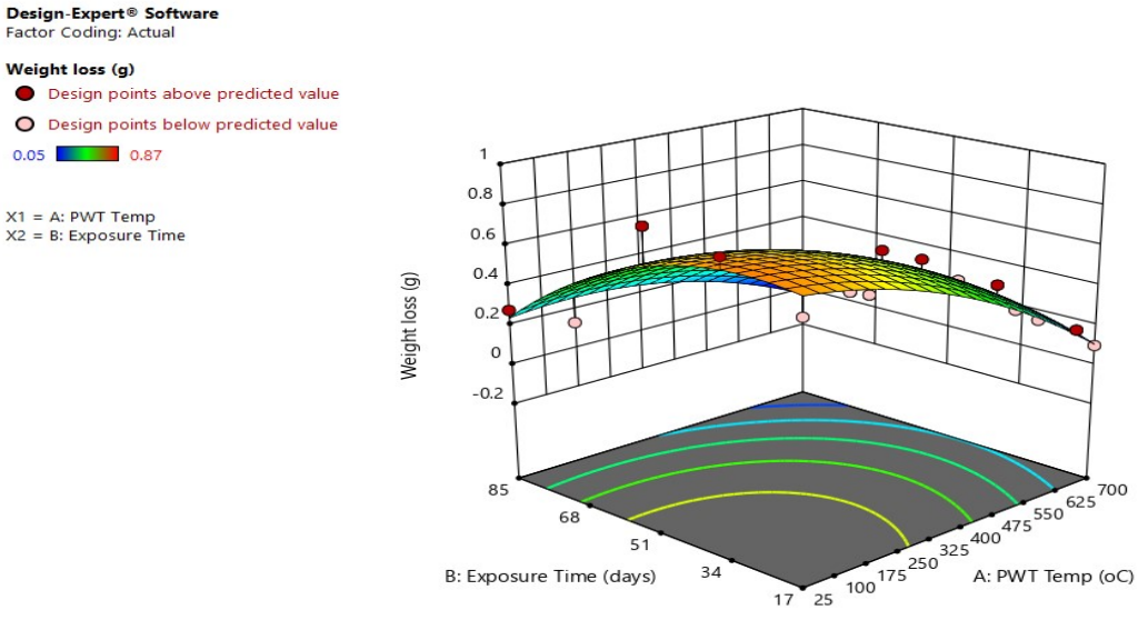
The study demonstrated a positive correlation between WL and CR, which has increased when the post-weld tempering T and ET decreased. CS metal dissolution retardation was due to the formation of a protective coating on its surface 38. Optimal conditions predicted from RSM on the effect of post-weld tempering and ET of CS are 25 ºC (as-welded) and 17 days of ET, and ideal WL and CR were predicted to be 0.744 g and 0.768 mm/yr, respectively. This shows that post-weld tempering is an effective method for improving corrosion properties of CS in a Sw environment.
Validation of optimum parameters
To confirm the data validity, an additional experiment was conducted, as presented in Table 5. Experimental WL and CR values of 0.760 g and 0.798 mm/yr were close to the predicted values of 0.744 g and 0.769 mm/yr, respectively. UE for WL and CR were 1.6 and 2.9%. These values lower than 5% showed that the generated models adequately predicted WL and CR of welded and tempered CS in Sw.
Conclusion
The following conclusions can be deduced from this study. The optimal conditions for maximum WL and CR of UNS G10400 CS occurred at 25 ºC (as-welded), with an ET of 17 days. Optimal values for WL and CR were 0.744 g and 0.769 mm/year, respectively. This shows that post-weld tempering was an effective method for improving corrosion properties of welded CS in a Sw environment.
ANOVA results of quadratic regression model used to fit the response revealed that it was significant (p< 0.0001). F-values and R2 showed good statistical agreement between experimental and predicted values. This is an expression of the model degree of significance and fitness.
Validation of the optimized predicted results showed an UE of 1.6 and 2.9%, for WL and CR, respectively. This revealed that the generated model adequately predicted CP of welded and tempered CS in a Sw environment. The developed model can be effective in predicting appropriate output for welded and tempered UNS G10400 CS structures in a Sw environment.
Declaration of conflicting interests
The authors declare that there is no potential conflict of interest with respect to the research, authorship, and/or publication of this article.
Authors’ contributions
Benjamin U. Oreko, Silas O. Okuma: conceptualized the research, drafted the manuscript, reviewed it and wrote its final version. Silas O. Okuma: carried out the experiments.
Abbreviations
ANOVA: analysis of variance
CCD: central composite design
CP: corrosion parameters
CR: corrosion rate
CS: carbon steel
CV: coefficient of variation
DF: degree of freedom
ET: exposure time
F: failure
GC: gravimetric corrosion
GT: gravimetric techniques
PWHT: post-weld heat treatment
PWT: post-weld tempered
R2: coefficient of determination
RSM: response surface methodology
SD: standard deviation
SNR: signal to noise ratio
Sw: seawater
T: temperature
UR: uncertainty error
WL: weight loss

