


 Inglês (pdf)
 Artigo em XML
 Referências do artigo
 Enviar este artigo por email
 Citado por SciELO
  Similares em
SciELO
Similares em
SciELO 
 Permalink
Introduction
Decomposition of organic wastes in an oxygen-free environment requires anaerobic microorganisms, which feed on the nutrients it contains, thereby converting it to biofuel. The development of several microbial growth kinetics model has helped explaining this process. Inherent to most models, such as Andrew, Contois, Monod, Moser and Verhulst, are independent factors like biomass and SC, in the bioreactor under consideration, where the microorganism’s SGR is the output variable. Since exponential microbial growth plays a key role in organic waste conversion, in most environmental engineers’ agenda it is crucial to optimize their development, especially during biodegradable waste anaerobic decomposition. Kinetic models have been employed in recent years, of which parameters were used to predict biogas optimal production and the growth rate of isolated microbes that help digesting feedstock. Others scholars have employed RSM to generate DOE, proposing different combinations of input variables for single or sets of responses or outputs. Currently, NN predictive modeling has evolved as a new optimization tool in bioprocessing, for biogas yield prediction, with random combination of factors, from palm oil mill effluents, cassava wastewater, cow dung and food waste, etc., using MATLAB 2,3,9,12.
Thorough research shows that prior studies using typical microbial growth kinetic parameters for biomass and SC are non-existent, especially a practical application of JMP software 7 linked to the anaerobic process. Applying NN predictive modeling technique to banana peels and chicken manure anaerobic decomposition can provide valuable insights onto processing behavior and enhance its management, leading to more efficient and reliable biogas and biofertilizer production. This study aimed to: use two different digesters separately charged with Sample A (banana peels + chicken manure) and Sample B (chicken manure) for microbial growth study; mathematically and experimentally determine and generate a dataset for the respective depleting Ct of SC and biomass in the exponential growth phase in their respective chambers, to calculate their microbes SGR; use datasets distinctly recorded in JMP software, specifying an orthogonal CCD, before programming it to generate a neural predictive model; analyze SGR statistical outputs of Sample A and B, for training and validation fitted plots; employ OriginPro 2018 software for a user-defined regression analysis, specifying the Monod equation, to estimate kinetic parameters for each dataset; and compare fits, surface plots, kinetic parameters and the predictive model for the two datasets, to determine the optimal combination of input variables. Similar to this work, 8 have carried out a combined demonstration of kinetics (using modified Gompertz model) and ANN, for biogas production via anaerobic digestion observations. 5 have also examined the behavior of biogas yield curve from lignocellulosic material using ANN. The present study suggests a different and more enhanced approach of merging the idea behind regression, CCD for RSM and neural modeling, to achieve the stated goals.
Methodology and materials
Materials sourcing
Banana peels and chicken manure were collected from Kasuwan Shanu Market and UNIMAID Faculty of Agriculture Poultry Farm, respectively, both in Maiduguri, Borno State, Nigeria. Drinkable water was utilized for anaerobic digestion and cell density determination. Before digestion, organic biomass was processed into Sample A and Sample B. Sample A is a mixture of chicken manure (4 kg), banana peels (0.5 kg) and water (7.5 kg) in a digester. Sample B is a mixture of chicken manure (7.5 kg) and water in equal proportions by weight, decomposed in a different digester. The two digesters were operated in batch mode, as described by 17.
Biomass and SC datasets
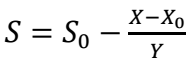
Viable cells in samples A and B digesters were determined using hypothetical units- colony-forming units (CFU/mL) converted to SC in mg/L units. In microbiology and cell growth experiments, biomass means the viable cells counted in colonies, which stand as Ct from biomass. This determination was carried out by manual NA preparation. From the experiment onset, it was assumed that chicken manure contains microorganisms which are paramount to the anaerobic process (10). Using a biomass-to-SC ratio of Y = 400, SC was determined using Eq. 1 (1) for samples A and B, respectively.
 (1)
(1)
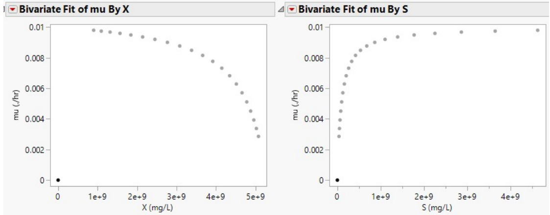
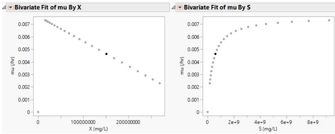
Depletion of nutrients or feedstock by biomass during anaerobic fermentation, or the feedstock amount left at a particular time, are typified as S. In Eq. 1, X0 and S0 represent initial biomass and SC, which are 899868717.4 and 4620000000 mg/L, (Sample A), and 15351147.09 and 9232210402.48 mg/L, respectively (Sample B). By convention, µ and S in Monod plots are often extracted from the growth phase of the microorganism acting on the samples. Hence, datasets for S and 𝜇 are inverted, initiating at S = 0 and 𝜇 = 0, before plotting Monod curve (Figs. 1 and 2 (b)).
RSM
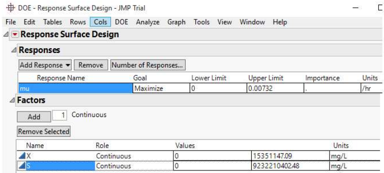
JMP® Trial 17.2.0 (701896), Serial Number: T-VHFY3P0J09 was installed on Microsoft Windows 10 Pro (10.0.10240.0). The software was developed by JMP Statistical Discovery LLC, by Neil Hodgson (neilh@scintilla.org). Under DOE menu, and Classical drop-down menu, Response Surface Design was selected. For RSM analysis of Sample A and B, the response (µ), called SGR (h-1) was to be maximized. The specification of upper and lower limits of X and S factors is shown in Figs. 3 and 4.
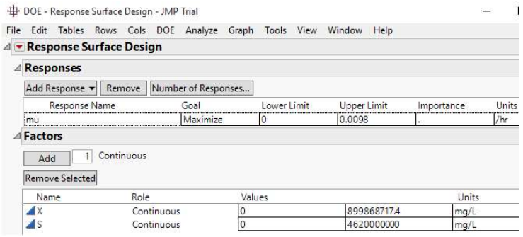
Then, CCD-Orthogonal Design Type, over 16 runs and 8 center points, was chosen, and a randomized output option run order was selected. A table of the runs that was generated by JMP was then assessed for implementation. If the estimates of X and S given in the table are not realistic, those empirically obtained (Figs. 1 and 2) are entered after JMP proposed outcomes are deleted.
Incorporating a NN design
Using sets of empirical X, S and µ, which were used to visualize microbial growth via Figs. 1 and 2, NN was generated for µ outcomes. To do that, NN was selected under ‘Predictive Modeling’ drop-down arrow, under “Analyze” menu in JMP application. NN is a modern predictive modeling technique that predicts the response variable, using a flexible function of input variables (e.g., X and S). The respective factors and the response were then chosen, and a Random Seed of 0 was defined, to generate a reproducible sequence of random numbers, starting from 0. In Model Launch window, a Holdback Validation Method used to assess the performance of a trained model was selected. A default Holdback Proportion of 0.333, referring to a fraction of the dataset reserved for validation/testing purposes, or a determinant of how the dataset is split into training, validation and test sets, were allowed, as conducted by 9. Afterwards, 3 was entered as the number of hidden nodes, and the model was launched using ‘Go’ button.
Expected results after the model run were: samples A and B dataset statistical parameter estimates; NN; prediction profiler model interpretation and sensitivity analysis representations; 3D surface profiles 16; Actual by Prediction plots; a table containing formulas for the predicted response and hidden layers’ nodes; and SAS code that can be used to score a new dataset. Using prediction profiler, optimal settings for predictor variables that led to desired predicted outcomes were found, in order to optimize the process. Based on 40 experimental runs, JMP simulated several DOE for microbial growth process involving X, S and µ average estimates.
Results and discussion
Training/validation and statistical measure based on predicted µ
A holdback validation method is a crucial technique for assessing and fine-tuning NN models, which helps to prevent overfitting, and ensure they generalize well to new and unseen data. A holdback of 0.333, as specified, implies that 66.7% of the data were allocated for training, while 33.3% was set aside for validation or testing. Commonly, the specific choice of the holdback proportion depends on the nature of the problem, the dataset size, and the goals of the machine learning experiment. In the regression analysis context, R2 is a metrics often used for training and validation datasets 3,13. Higher R2 of 0.9888 and 1.0000 for training, and lower R2 of 0.9788 and 0.9999 for validation, obtained for Samples A and B statistical metric (Table 1), respectively, indicated overfitting.
Table 1: Sample A and B statistical model fitting predictions.
| Measure | Sample A | Sample B | ||
|---|---|---|---|---|
| Training value | Validation value | Training value | Validation value | |
| R2 | 0.9887916 | 0.9787637 | 1 | 0.9999999 |
| RASE | 0.0002279 | 0.0004126 | 1.8517 x 10⁻⁷ | 4.8578 x 10⁻⁷ |
| Mean abs dev | 0.0001933 | 0.0002962 | 1.5785 x 10⁻⁷ | 4.2239 x 10⁻⁷ |
| -Log likelihood | -97.5472 | -50.99224 | -225.3291 | -104.9486 |
| SSE | 7.2715 x 10⁷ | 1.3621 x 10⁻⁶ | 5.486 x 10⁻⁷ | 1.888 x 10⁻¹² |
| Sum freq | 14 | 8 | 16 | 8 |
Overfitting occurs when the model is able to perfectly fit training data, but fails to generalize them to unseen data. In such cases, the model may capture noise and idiosyncrasies in training data, which results in high R2 value for training. When applied to validation dataset, the model performs poorly, resulting in lower R2 value. Viz-a-viz, higher R2 for validation and lower R2 for training are often a sign of underfitting. However, if R2 values for both training and validation are reasonably high and close to each other, as shown in Table 1, this indicates that the model is able to capture underlying patterns in the data without overfitting or underfitting 6. SSE can be explained in terms of training and validation. Training SSE close to zero implies that the model is perfectly fitting training data, while lower validation SSE indicates better generalization. Clearly, results in Table 1 establish an ideal scenario, where validation SSE is reasonably close to the training one, for the respective samples, it shows that the model learnt underlying patterns in the data without overfitting. Similarly, lower training RASE of 0.0002279 (Sample A) and 1.8517 x 10⁻⁷ (Sample B), shows that the model predicted training data with smaller errors.
MAD or MAE behavior, which quantifies how far predictions are from true values on average, is consistent whether one is looking at training or validation dataset. If R2 is high for training dataset, MAD will typically be lower on it (e.g., 0.0001933 for Sample A). Alternatively, low R2 for validation dataset will result in higher MAD on validation dataset (viz. 0.0002962). As for equal R2 (dataset B), MAD’s estimates can be used to select models. In order to minimize prediction errors in practical applications where accuracy is crucial, lower MAD (i.e., 1.5785 x 10⁻⁷ for training) is suitable. Sum of frequencies show how many data points are present in each dataset, which is crucial in assessing reliability and generalizability of NN predictive model. Larger datasets (as in Sample B) are often beneficial for training more robust and accurate models. The difference itself in “Sum Freq” between training and validation datasets does not inherently indicate an issue. “Loglikelihood” is a term used to quantify how well a statistical model’s predictions match observed data, in which lower values (i.e., -97.5472 and -225.3291 for Samples A and B training, respectively) indicate a better fit.
Hidden layers’ structure
In a NN, hidden nodes, as earlier specified in the methodology, are computational units that are part of hidden layers, which stand between input (X and S blue box) and output layers (𝜇 square box), as shown in Fig. 5.
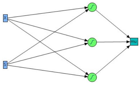
Hidden nodes are responsible for processing input data and learning complex patterns and representations from them 2. Hidden layers with 3 hidden nodes mean that this layer contains 3 computational units. The units in the green field circle containing ‘S’ symbol, as shown in Fig. 5, are called TanH (14).
Due to selected alike nodes, Fig. 5 is similar for samples A and B data. Changing the number of hidden nodes from 3 to 5 and 10, for Sample A dataset, will affect the extent of fit and R2 values 4,11. At hidden nodes of 3, 4 and 5, R2 values were: for training, 0.9887916, 0.9678015 and 0.9926753; and for validation, 0.9787637, 0.9786579 and 0.9786468. Initially, increasing hidden nodes number might lead to an improvement in R2 for training dataset, since a more complex model is able to learn intricate patterns on data. Further increase in nodes (to 10) will lead to overfitting, as the model starts to fit noise or random variations in training data, which results in artificially high R2. Likewise, increasing hidden nodes may, at first, improve R2 for validation dataset, because the model can capture more nuances in data. Nevertheless, if the model starts to overfit training data, R2 for validation dataset is likely to decrease. Generally, increasing the hidden nodes number can affect the dependent variable (µ) prediction. NN with more hidden nodes is computationally more complex, and it may require additional computational power and memory. What is called “black box” may occur 2, a situation in which it has signally became challenging to interpret how specific features or variables impact µ, due to more hidden nodes.
Prediction profile under maximum desirability
In JMP software, prediction profiler is a tool used for exploring and visualizing X and S effects on predictions made by a statistical model. It is particularly useful for understanding how changes in input variables (predictors) impact predicted outcome (µ) from the model. As portrayed in Figs. 6 and 7, desirability refers to a measure used to assess the overall quality of a set of predicted outcomes for a given set of input conditions or factors.
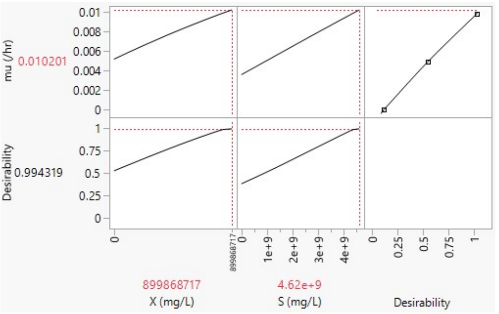
In Fig. 6, a high desirability score of 0.994319 indicates that a combination of X = 899868717 mg/L and S = 4.62 x 10⁹ mg/L led to optimal or desirable values of µ = 0.010201 h-1, which met the desired goal. This is because, when working with prediction profilers and desirability, the aim is to find factor settings or input conditions that maximize overall desirability score.
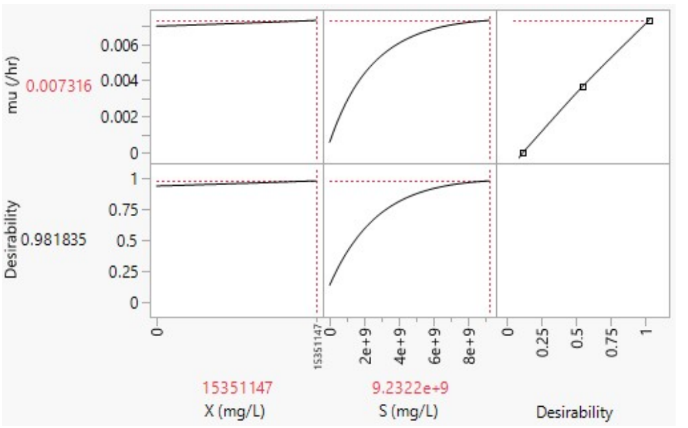
Hence, in the same context, X = 15351147 mg/L and S = 9.2322 x 10⁹ mg/L, which, at high desirability of 0.981835, is the desired combination for µmax of 0.007316 h-1 (Fig. 7).
Simulation experiment
‘Simulation’ feature, under prediction profiler in JMP software, was used to perform Monte Carlo simulations, for predicting X and S values, and statistical properties: mean and SD of µ for 40 experimental runs (Tables 2 and 3).
Table 2: JMP predicted experimental runs for sample A dataset.
| Run | X (mg/L) | S (mg/L) | µ mean (h) | µ SD |
|---|---|---|---|---|
| 1 | 830648046.83 | 3968461538.50 | 0.008959737 | 1.21E-17 |
| 2 | 819111268.40 | 2310000000.00 | 0.006560012 | 1.04E-17 |
| 3 | 888331938.97 | 3613076923.10 | 0.008731199 | 1.21E-17 |
| 4 | 784500933.12 | 4027692307.70 | 0.00881895 | 1.21E-17 |
| 5 | 461471137.13 | 3316923076.90 | 0.00617417 | 1.65E-17 |
| 6 | 634522813.55 | 3020769230.80 | 0.006670966 | 2.60E-18 |
| 7 | 530691807.70 | 3790769230.80 | 0.007191932 | 1.04E-17 |
| 8 | 484544693.98 | 3139230769.20 | 0.00605546 | 8.67E-18 |
| 9 | 669133148.84 | 2783846153.80 | 0.006513329 | 1.73E-18 |
| 10 | 449934358.70 | 2606153846.20 | 0.005140131 | 0 |
| 11 | 611449256.69 | 4383076923.10 | 0.008428288 | 1.21E-17 |
| 12 | 715280262.55 | 4501538461.50 | 0.009129081 | 2.43E-17 |
| 13 | 599912478.27 | 4560769230.80 | 0.00860883 | 2.26E-17 |
| 14 | 646059591.98 | 3198461538.50 | 0.006976319 | 1.73E-17 |
| 15 | 703743484.12 | 3435384615.40 | 0.007595131 | 1.91E-17 |
| 16 | 576838921.41 | 3080000000.00 | 0.006458603 | 1.73E-18 |
| 17 | 807574489.97 | 4146153846.20 | 0.009096647 | 1.21E-17 |
| 18 | 519155029.27 | 3909230769.20 | 0.007291284 | 1.73E-17 |
| 19 | 876795160.54 | 2487692307.70 | 0.007076688 | 5.20E-18 |
| 20 | 796037711.55 | 4620000000.00 | 0.009698155 | 1.56E-17 |
| 21 | 772964154.69 | 2428461538.50 | 0.006513781 | 1.65E-17 |
| 22 | 692206705.69 | 2369230769.20 | 0.006043987 | 1.56E-17 |
| 23 | 565302142.98 | 2902307692.30 | 0.006153266 | 8.67E-19 |
| 24 | 507618250.84 | 3257692307.70 | 0.006340537 | 1.04E-17 |
| 25 | 588375699.84 | 4323846153.80 | 0.008225424 | 0 |
| 26 | 865258382.12 | 4205384615.40 | 0.009456864 | 0 |
| 27 | 542228586.13 | 2961538461.50 | 0.006115486 | 8.67E-18 |
| 28 | 853721603.69 | 2665384615.40 | 0.007225682 | 6.07E-18 |
| 29 | 473007915.56 | 3731538461.50 | 0.006800266 | 3.47E-18 |
| 30 | 899868717.40 | 3553846153.80 | 0.008700551 | 1.21E-17 |
| 31 | 657596370.41 | 4086923076.90 | 0.008263504 | 1.21E-17 |
| 32 | 680669927.26 | 4264615384.60 | 0.008626408 | 1.21E-17 |
| 33 | 622986035.12 | 3672307692.30 | 0.007514357 | 1.73E-17 |
| 34 | 761427376.26 | 4442307692.30 | 0.009280284 | 1.21E-17 |
| 35 | 553765364.55 | 2843076923.10 | 0.006011707 | 1.56E-17 |
| 36 | 749890597.83 | 3376153846.20 | 0.007739604 | 1.13E-17 |
| 37 | 496081472.41 | 3850000000.00 | 0.00708624 | 0 |
| 38 | 842184825.26 | 2546923076.90 | 0.007003912 | 1.73E-17 |
| 39 | 738353819.41 | 2724615384.60 | 0.006768006 | 1.04E-17 |
| 40 | 726817040.98 | 3494615384.60 | 0.007792039 | 1.91E-17 |
Higher number of runs provides more precise estimates of µ’s mean and SD. The relationship between µ and limiting S given in the tables, over 40 runs, can be described using Monod equation (Eq. 2), for a typical controlled microbial environment to which Samples A and B were subjected to.
 (2)
(2)
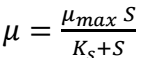
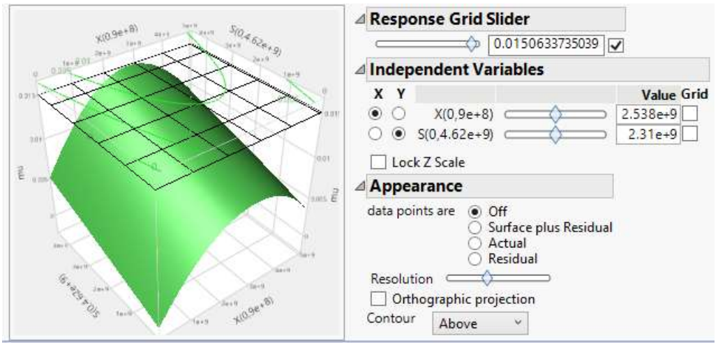
where µmax is maximum SGR, i.e., rate at which microorganisms can grow when S is not limiting, and Ks is half-saturation constant or S, at which µ is half of µmax. Since there are no estimates of µmax and Ks, to aid selecting an optimal design, a run with higher µ in Tables 2 and 3 may hint on X and S best combinations. Thus, Sample A dataset’s X = 899868717.4 mg/L and S = 4.62 x 10⁹ mg/L (Table 2), at µmax = 0.009698155 h-1 below maximum desirability, as shown in Fig. 6. On the other hand, Sample B dataset’s X = 15351147.09 mg/L and S = 9232210402.5 mg/L (Table 3), at µmax of 0.00728 h-1 below maximum desirability, as shown in Fig. 7, since estimates were not practically experimented and compared with the ones given by JMP.
Table 3: JMP predicted experimental runs for sample B dataset.
| Run | X (mg/L) | S (mg/L) | µ mean (h) | µ SD |
|---|---|---|---|---|
| 1 | 14367099.20 | 7811870340.60 | 0.007152 | 5.67255E-16 |
| 2 | 13776670.47 | 5562998575.90 | 0.006648 | 1.76074E-16 |
| 3 | 12005384.26 | 8166955356.00 | 0.00713 | 6.65267E-16 |
| 4 | 8856431.01 | 8640402043.30 | 0.007108 | 5.73326E-16 |
| 5 | 8659621.44 | 7456785325.10 | 0.006924 | 1.04951E-16 |
| 6 | 13383051.31 | 6864976965.90 | 0.006965 | 2.6975E-16 |
| 7 | 11808574.69 | 5918083591.30 | 0.006676 | 4.25875E-16 |
| 8 | 9053240.59 | 5089551888.50 | 0.006274 | 5.96745E-16 |
| 9 | 12989432.15 | 6509891950.50 | 0.006875 | 6.24501E-16 |
| 10 | 8266002.28 | 8877125387.00 | 0.007122 | 9.28077E-17 |
| 11 | 7872383.12 | 8522040371.50 | 0.007069 | 1.08507E-15 |
| 12 | 10627717.22 | 5326275232.20 | 0.006433 | 1.40599E-15 |
| 13 | 10824526.79 | 8995487058.80 | 0.007193 | 1.1163E-15 |
| 14 | 14170289.62 | 5799721919.50 | 0.006737 | 1.0365E-15 |
| 15 | 15154337.51 | 7930232012.40 | 0.007191 | 1.97759E-16 |
| 16 | 10234098.06 | 7575146996.90 | 0.006993 | 1.81105E-15 |
| 17 | 8462811.86 | 7220061981.40 | 0.006873 | 2.09902E-16 |
| 18 | 9250050.17 | 6154806935.00 | 0.006645 | 7.61544E-16 |
| 19 | 11611765.11 | 5681360247.70 | 0.006596 | 7.31186E-16 |
| 20 | 15351147.09 | 8758763715.20 | 0.00728 | 1.5786E-16 |
| 21 | 13973480.04 | 4852828544.90 | 0.006397 | 1.7486E-15 |
| 22 | 12595813.00 | 6273168606.80 | 0.006803 | 6.03684E-16 |
| 23 | 13579860.89 | 5444636904.00 | 0.006601 | 8.92515E-16 |
| 24 | 14957527.93 | 8285317027.90 | 0.007225 | 9.6971E-16 |
| 25 | 13186241.73 | 6983338637.80 | 0.006982 | 1.81279E-15 |
| 26 | 11414955.53 | 7101700309.60 | 0.006945 | 1.00614E-16 |
| 27 | 12792622.58 | 8048593684.20 | 0.007137 | 2.09902E-16 |
| 28 | 14563908.78 | 6628253622.30 | 0.006959 | 6.21031E-16 |
| 29 | 12202193.84 | 7693508668.70 | 0.007071 | 1.39559E-15 |
| 30 | 7675573.55 | 8403678699.70 | 0.007049 | 1.47452E-17 |
| 31 | 9643669.33 | 4616105201.20 | 0.006094 | 1.44503E-15 |
| 32 | 9446859.75 | 6746615294.10 | 0.006803 | 1.29931E-15 |
| 33 | 14760718.36 | 6391530278.60 | 0.006914 | 4.42355E-17 |
| 34 | 11021336.37 | 6036445263.20 | 0.006679 | 1.31319E-15 |
| 35 | 12399003.42 | 9232210402.50 | 0.007249 | 1.13798E-15 |
| 36 | 9840478.90 | 4971190216.70 | 0.00626 | 2.8276E-16 |
| 37 | 10430907.64 | 4734466873.10 | 0.006184 | 1.5786E-15 |
| 38 | 11218145.95 | 9113848730.70 | 0.007213 | 5.67255E-16 |
| 39 | 10037288.48 | 7338423653.30 | 0.006945 | 1.3262E-15 |
| 40 | 8069192.70 | 5207913560.40 | 0.006279 | 1.12497E-15 |
Surface profile
Just as previously demonstrated by 11,15, predictors’ (S and X) effect on the response can be simulated with NN model, and analyzed using 3D surface plots. Fig. 8 shows that µ increased gradually with X, before attaining µmax of 0.015 h-1, and then declined, after nutrients became low. Likewise, µ increased as S decreased and X rose, as shown in Fig. 9.
Fitted plots and model equation command code
In the specified fit, plot for training set with actual and predicted values on Y- and X-axes, respectively, and validation set are shown in Figs. 10 and 11. They are generated by JMP based on their number of data points or Sum Freq. or counts given earlier in Table 1.
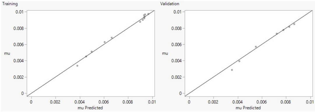
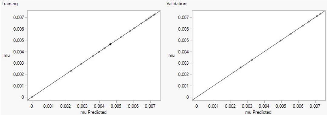
Under training linear fitting plots in both figures, random data splitting process instigates more data points, to end up in the training dataset by chance. As previously described, MAD and R2 are complementary metrics. High and low R2 often correspond to lower and higher MAD, indicating better and worse model fits, respectively (Fig. 10a and b). Fig. 11, for chicken manure model fitting of µ, shows that R2 values for training and validation datasets are equally high (Table 1). This suggests that the model performed well in terms of explaining the variance in the target variable, and generalized effectively to unseen data 9. This is actually a positive sign. However, if precise and accurate predictions are the analysis’ priority, the training model with less errors (SSE = 5.486 x 10⁻¹³) should be chosen based on its lower MAD. A model with higher MAD (validation) should be selected if one wishes more sensitivity to potential outliers or extreme cases. Another reason for better fit in both training graphs is that their negative log-likelihoods are lower, while higher values in validation plots suggest poorer fit 7.
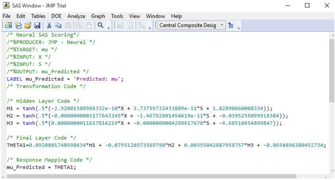
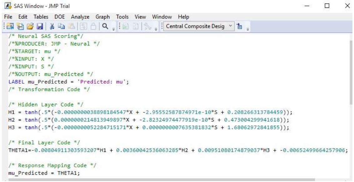
Figs. 12 and 13 depict Ntan(H) model equations for 3 hidden layers. Notably, 13 utilizes 2 hidden layers and both neural and fuzzy logic to optimize biogas yield from datasets of two reactor setups TanH function’s advantage is that it is nonlinear, allowing to map more intricate functions and stack layers, and to obtain high precision 14.
Experimental versus predicted 𝛍 datasets
In samples A and B (Figs. 14 and 15), increased µ means microbial growth faster rate, which rapidly depletes S, as it further consumes the substrate. In that case, µ in Monod equation represents microbial growth in relation to limiting S. Predicted values (Figs. 14 and 15), using model equations in Figs. 12 and 13, showed almost 100% fit demonstrated by the earlier shown plots. When regression was performed using OriginPro 2018 software, µmax and Ks values obtained for experimental and predicted samples were almost equal (Table 4). Although model equation for predicted µ of A dataset indicated that it was reliable, resulting in values of µmax = 0.00997 h-1 and Ks = 9.12975 x 10⁷ mg/L (0.01 h-1 and 9.498595 x 10⁷ mg/L), the same parameters estimated for experimental results gave the best combination, coupled with their corresponding X and S based on maximal desirability. Model equation for Sample B accurately mimicked Eq. 2, since it gave 100% equal experimental and predicted µmax and Ks (0.00762 h-1 and 3.838 x 10⁷ mg/L, respectively) values and suitable chicken manure data (Fig. 13). These parameters, along with X and S maximal desirability (Fig. 7), indicate that Sample B study was the optimal combination.
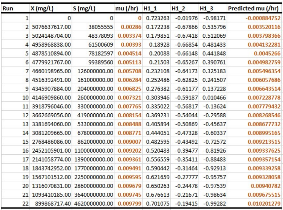
Constant "H" in Figs. 14 and 15, as herein mentioned, likely represents a parameter in model equations used for predicting µ of microorganisms based on X and S input variables. Positive "H" constant may suggest that certain conditions or factors it represents have a stimulatory effect on microbial growth, and indicate a direct relationship with µ, meaning that they increased together. Conversely, negative "H" constant may imply inhibitory factors or conditions that negatively impact microbial growth, which indicates an inverse relationship with µ. In this case, as "H" value decreased, µ increased.
Parameters, such as µmax and Ks allow scientists to predict how fast microbial growth is under specific nutrient Ct. It is quite important in this study, since µ specifically impacts biogas generation, when Sample A or B are used, with their associated production rates.
Optimization of S in their respective bioreactors to maximize microbial growth is aided with the knowledge of these parameters. In the Monod equation, an increase in µmax would lead to a higher 𝜇 that can be achieved under optimal conditions. An increase in µmax implied higher microbial growth potential, which could lead to faster substrate consumption and, consequently, a decrease in S, over time 1.
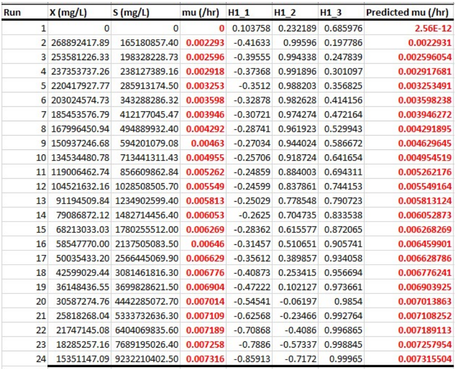
Table 4: Statistics and estimated Monod parameters.
| Sample A | Sample B | |||
|---|---|---|---|---|
| Experimental | Predicted | Experimental | Predicted | |
| Number of points | 22 | 22 | 24 | 24 |
| Degrees of freedom | 20 | 20 | 22 | 22 |
| Reduced chi-square | 4.98155E-12 | 1.01704E-07 | 1.06662E-19 | 4.54345E-14 |
| Residual sum of squares | 9.46310E-11 | 2.03408E-06 | 2.34655E-18 | 9.99560E-13 |
| R2 (COD) | 1 | 0.98769 | 1 | 1 |
| Adj. R2 | 1 | 0.98707 | 1 | 1 |
| Fit status | Succeeded (100) | Succeeded (100) | Succeeded (100) | Succeeded (101) |
| µmax (h-1) | 0.01 | 0.00997 | 0.00762 | 0.00762 |
| Ks (mg/L) | 9.49859E + 07 | 9.12975E + 07 | 3.838E + 08 | 3.83747E + 08 |
Conclusion
R2 values near or equal to 1, obtained on training and validation sets, show that TanH neural models for Samples A and B datasets correctly predicted µ. Under 99.43% desirability score, µmax of 0.01 h-1 and Ks of 9.498595 x 10⁷ mg/L, the combination of X and S (899868717 mg/L and 4.62 x 10⁹ mg/L, respectively), for optimal µ of 0.010201 h-1, was valid for Sample A’s experimental observations. Estimated Monod parameters for µmax and Ks (0.00762 h-1 and 3.838 x 10⁷ mg/L, respectively), based on 98.18% desirability for X and S (15351147 and 9 x 10⁹ mg/L), made optimal microbial growth condition that resulted in maximum µ of 0.007316 h-1, which was valid for Sample B empirical and predicted outputs. Overall, Sample B’s anaerobic chamber produced higher biogas yields that those from Sample A’s bioreactor. This was due to exact R2 and kinetic parameter values obtained for experimental and forecasted 𝜇. In future researches, neural predictive modeling of two datasets, employing linear and Gaussian representative models, can be run using JMP, of which outcome may be compared with estimates in this study and with the created TanH equation. In addition, hidden nodes variation may improve R2 estimation and predicted values, especially for Sample B estimates, which still falls below observed variables and obtained parameters. Applying advanced statistical tools like JMP and NN allows for data-driven decision making, which can result in optimized process parameters and improved waste-to-resource conversion.
Declaration of interests
Authors declare that they have no known competing financial interests or personal relationships that could have appeared to influence the work herein reported.
Authors’ contributions
A. M. Abubakar: study conceptualization; integrated new ideas with existing literature; analyzed results using JMP and OriginPro; studied and discussed results. N. Elboughdiri: carried out literature survey; reviewed and edited the manuscript; provided project administration and support. A. Chibani: chose the research problem; gave outlines for the manuscript preparation. E. C. Nneka and D. Ghernaout: reviewed and edited the manuscript; guided the paper writing. M. U. Yunus: completed experimental part; helped in raw material sourcing.
Abbreviations
ANN: artificial neural network
CCD: central composite design
COD: coefficient of determination (R2)
DoE: design of experiment
MAD: mean absolute deviation
MAE: mean absolute error
NA: nutrient agar
NN: neural network
RASE: root average squared error
RMSE: root mean square error
RSM: response surface methodology
SAS: statistical analysis system
SC: substrate concentration
SD: standard deviation
SGR: specific growth rate
SSE: sum of squared errors
TanH: hyperbolic tangent

