Modeling and forecasting foreign direct investment into Brazil with ARIMA

Frederico Araújo Turolla* & Mário Antônio Margarido**

 

*Doutorado em Economia de Empresas, Fundação Getúlio Vargas de São Paulo (FGV-SP). Professor Associado, Mestrado em Gestão Internacional, Escola Superior de Propaganda e Marketing (ESPM), Brasil. E-mail: fturolla@espm.br

**Doutorado em Economia Aplicada, Universidade de São Paulo (USP). Pesquisador Científico, Instituto de Economia Agrícola de São Paulo (IEA-SP), Brasil. E-mail: mamargarido@iea.sp.gov.br

 

ABSTRACT

In this paper we have tested the hypothesis that the Foreign Direct Investment (FDI) flows into Brazil have a Moving Average pattern in line with predictions from the theory. We have modeled the FDI series in US dollars using a univariate model, the Auto-Regressive Integrated Moving Average (ARIMA) model. The results confirmed the hypothesis derived from the theory that, after correcting for detected outliers, there is a Moving Average pattern in FDI inflows into Brazil as there is quite a dynamic series with relatively rapid adjustment towards equilibrium values. The patterns found can be used in univariate modeling to generate forecasts of the future values of the series. We present a forecast for the series and discuss the issue of forecast accuracy using the Theil Coefficient.

Key words: Internalization Theory, Foreign Direct Investment, ARIMA Model, Intervention Analysis

 

Modelagem e previsão do investimento direto no Brasil com ARIMA

RESUMO

Neste artigo, foi testada a hipótese de que os fluxos de Investimento Direto Estrangeiro (IDE) para o Brasil apresentam um padrão de Médias Móveis, em linha com as previsões da teoria. Foi modelada a série de IDE em dólares norte-americanos usando um modelo univariado, o Auto-Regressive Integrated Moving Average (ARIMA). Os resultados confirmaram a hipótese derivada da teoria de que há um padrão de Médias Móveis no IDE no Brasil, na medida em que se trata de uma série bastante dinâmica com ajustamento relativamente rápido em relação aos valores de equilíbrio. Com base no padrão identificado, o trabalho também mostrou a possibilidade de geração de previsões de fluxos de IDE e apresentou uma previsão, discutindo a questão de exatidão de projeções usando o coeficiente de Theil.

Palavras-chave: Teoria de Internalização, Investimento Direto Estrangeiro, Modelo ARIMA, Análise de Intervenção

 

INTRODUCTION

Quantitative modeling of foreign direct investment (FDI) flows is relevant for empirical verification of the various competing approaches in the field of international business; for informed policy making on FDI and other related aspects; and for financial market uses in the anticipation of the specific component in the balance of payments, which is often used in exchange rate forecasts and economic scenarios in general.

In addition, the observation of empirical regularities may lead to a reassessment of the predictions of existing theories. This is especially valuable for the study of idiosyncrasies of specific countries for which long historical data sets are available. Although such an approach at an aggregate level may lack some important points of the theory that are quite firm-specific, the assessment of the univariate properties of the FDI series leads to a better understanding of its underlying data generation process.

In light of this importance, this paper concentrates on modeling the FDI flows into Brazil. Similar studies for other countries include Bashier and Talal (2007), for Jordan. One result of particular interest is that the pattern of the inward FDI into Brazil has a b moving average component of order 1, as described in the paper, in addition to other less prominent components. This suggests quite a dynamic economic variable, with fast adjustment against past errors. The model also allowed us to build a forecast of the variable’s future values.

 

METHODOLOGY

In this paper we test relevant theories by modeling the Brazilian inward FDI series in US dollars using an univariate model, the Auto-Regressive Integrated Moving Average (ARIMA) model such as the one proposed by Box, Jenkins and Reinsel (1994), with interventions as discussed in Box and Tiao (1975). The FDI series was named IDE. In this univariate model, the behavior of the variable at a given observation t is explained by its own past values (auto-regressive, AR terms) and by its own past and present errors (moving average, MA terms). The identification of the presence of outliers is an important feature of modeling. Given the specific pattern of the series, we have also carried forward a forecast of the future values of the FDI series that we have modeled. We present a discussion on the accuracy of the forecasts, using the Theil inequality coefficient approach, as in Theil (1966 and 1961).

 

THEORY

There are several competing explanations for foreign direct investment and its modes. The key explanations include the Uppsala model; the eclectic paradigm; and the internalization theory, all of which are briefly summarized below.

Johanson and Vahlne (1977) proposed what they have named an “establishment chain” for the internationalization of firms, based on their empirical observations of international subsidiaries of Swedish firms. They found that this establishment chain was set up according to the psychic distance (factors that make it difficult to understand foreign environments), in a dynamic but non deterministic process that evolves over time with learning and incremental commitment building, under a bounded rationality assumption. The same authors proposed an update of their theory, as recently presented in Johanson and Vahlne (2009). As Eden (2009) puts it, “outsidership relative to the relevant network, rather than psychic distance, is the root cause of uncertainty and precipitates the internationalization process” (Eden, 2009, p. 1409). In the original theory, liability of foreignness was a key concept whereas in the new version of theory the liability of outsidership becomes an important concept.

John Dunning (1977) and his so-called eclectic paradigm of international production emerged from the finding that the subsidiaries of American companies in the United Kingdom were more productive than similar firms in the US, even though America’s industrial productivity was much higher than in the UK. The Dunning paradigm is based on three components, ownership (O), location (L) and internalization (I), and so it can be named “OLI”. The ownership component is related to the firm-specific availability of resources and is associated to the Resource Based View (RBV) of the organization; the latter was proposed by Penrose (1959) who saw the firm as “a set of productive resources.” The RBV explains how companies manage to obtain a sustainable competitive advantage, analyzing their internal resources to correct their weaknesses and develop their potentials. The existence of assets – tangible or intangible – is linked to the firm’s capacity to expand and stand out from its competitors. Tangible assets include economies of scale or patents, while the firm’s brands and reputation are among its intangible assets. Dunning’s eclectic approach is criticized as too general, and was recently updated in Dunning and Lundan (2007).

The internalization theory of the multinational enterprise is a stream of literature initiated by Buckley and Casson (1976, 2003), as reviewed and updated by the same authors in Buckley and Casson (2009), hereafter B&C. The internalization approach is based on the Coasian nature of the firm in which imperfect markets can be internalized into firm’s internal non-market “transactions”. This approach raises the discussion of the firm’s boundaries, which “are set at the margin where the benefits of further internalization of markets are just offset by the costs”. In addition, firms seek the least-cost location for each activity considering relevant linkages, and R&D plays an important role in the firm’s profitability and growth (B&C, 2009).

However, elements of the Dunning paradigm coincide to some extent with the theories presented herein. For example, Buckley and Casson (2009) propose the view that internationalization occurs as a result of the interaction between internalization and location effects, which can be linked to Dunning’s L and I components, as they have influenced the development of the OLI paradigm.

The “I” component reflects a view that the boundaries of a firm should be directly related to the costs of the transactions in which that particular firm is actually involved. Ronald Coase (1937) argued that transaction costs are important to how the market is organized and this was subsequently extended by authors like Williamson (1985), who further developed the notion of the firm’s boundaries in presence of important market imperfections. The internalization component of the B&C approach to internationalization is very much based on this view.

It should be noted that Johanson and Vahlne (2009) also indicate a certain convergence between the dominant international business approaches as they urge researchers to look for “similarities between internalization theory/the OLI paradigm and their own network-based internationalization process model” (Eden, 2009, p. 1409). In fact, as Johanson and Vahlne (2009) propose that the firm should be viewed as an exchange unit rather than a production unit (Eden, 2009); they seem to converge with a Coase or Williamson approach. Thus, while there are competing international business theories, it can be anticipated that the ongoing convergence will lead to more unified explanations that have a b probability of success in light of the existing interfaces.

Important early refutations to the internalization theory were disputed by Buckley (1988) which is also part of other approaches to international production. One of these is of relevance to this paper, namely the possibility of testing the internalization theory through the examination of the aggregate pattern of foreign direct investments. For example, he noted that “it is possible that the activity observed is random, i.e., unsystematic. This can be easily dismissed by reference to the most simple data. These data show a high concentration of multinational activity by origin and by location” Buckley (1988, p. 186). In addition, he noted that

“… the crucial recent shift of the USA from being a net exporter of foreign direct investment to be a net importer would be explained by changes in the locational costs within the USA versus foreign locations at activity level (as mediated by the exchange rate) and by the impact of structural shifts in US domestic industry and their consequent impact on potential foreign investors in industries differentially affected by the changes in the relevant exogenous influences. The attractiveness of the US market and the difficulties of servicing it by other means than investment provide a market servicing-based explanatory adjunct” (Buckley, 1988, p. 190).

These comments suggest not only that location patterns matter, but also that there may a specific time-series pattern, which is neither random nor unsystematic. The above comment by Buckley (1988) in particular suggests that there may be a process of convergence in foreign direct investment inflows, i.e., current flows should be related to past flows if an equilibrium value is still to be reached. The ARIMA model is the kind of time series modeling that best represents such a time series which is moving towards equilibrium, in particular the moving average (MA) process described in the next section.

This paper addresses flows into the Brazilian economy, which will clearly not show stable equilibrium values given its transition nature after the comprehensive reforms implemented in the 1990s. By the end of the 1990s, FDI inflows into Brazil were equivalent to more than 5% of its GDP – a figure that is similar to what a typical developed economy received in the same period – whereas in the late 1980s Brazil used to receive less than 0.5% of its GDP in FDI inflows. If the theory is to be confirmed, MA process would be expected to best characterize the FDI inflows into Brazil. That is the hypothesis that we have tested in this paper using the data set and the econometric procedures described in the next section.

 

DATA SERIES AND ECONOMETRIC PROCEDURES

The series was the monthly total inflow of FDI (code 8199 of the Brazilian central bank’s Time Series Management System, available at http://www.bcb.gov.br/?timeseriessearch). A total of 178 observations were made each month between January 1995 and November 2009.

According to Box, Jenkins and Reinsel (1994), the behavior of a time series can be explained by its own past values (auto-regressive parameters AR) and by its present and past errors (moving average parameters MA):

where: represents the differentiated variable, centered against its respective average, while and are the auto-regressive and moving average polynomial of order and , respectively.

The ARIMA modeling procedure has four steps: 1) identification; 2) estimation; 3) verification; and 4) forecast. The procedure starts with model identification, where the original series has to be filtered so as to identify its generating process and make it stationary. The correlograms of the Auto Correlation Function (ACF) and the Partial Autocorrelation Function (PACF) were used to determine whether the data generating process is auto-regressive (AR) or moving-average (MA), and to ascertain the order of integration (I), and their respective orders. Following those procedures, the model can be estimated and the residuals are analyzed so as to assure the effectiveness of the earlier filtering process. The underlying hypothesis is that linear filters will result in white noise residuals, which are normal and independently distributed with zero mean and constant variance. Residuals verification can be performed by carrying out a test developed by Ljung and Box (1978), which is represented by the following equation

where:T = number of observations; = autocorrelation in lag . The null hypothesis is that all values amount to zero.

After the three preceding steps, the forecast model can be made. The accuracy of the forecast was measured using the Theil Inequality Coefficient, as in Theil (1966 and 1961). The starting point for this coefficient is the Average Square Error, hereafter EQM, defined as:

where: n =forecast value for period and = observed value in period .

Dividing EQM by the average of squares of observed values we have:

When , then , and in this case there is a perfect forecast. On the other hand, when , then , and the forecast is the worst possible. However, the Theil Inequality Coefficient is difficult to interpret. Using algebraic manipulation, the preceding equation allows the different sources of forecast errors to be determined using the Theil Inequality Coefficient, as follows:

where: p and a, represent the average of forecast and observed values, respectively; ^Sand ^S are the standard deviation of the forecast and observed values, respectively and is the coefficient of correlation between ^p and ^a.

The right side of (5) is divided in three components. The first component represents the squared difference between the average and forecast and observed values, and is termed Central Tendency Error or Bias of Averages. When averages coincide, errors are null. The second component is the squared difference between standard deviations of and ⁿ, and ^at represents Error of Unequal Variations or Bias of Variances. Finally, the third component is null when the correlation between ⁿ and ^at is direct and perfect ^(r=1), and it will be the maximum possible when the correlation is inverse and perfect, ^(r=1); this component is called Error of Imperfect Correlation.

Error Measures of each part have the same dimension as EQM; the percentage of each component is obtained by dividing each by EQM. Decomposing EQM allows the observation of the nature of forecast errors. Thus, we have

1) U^M= Proportion of the Bias of Averages , represented by:

2) U^s= Proportion of Bias of Variances:

3) U^c= Proportion of Imperfect Correlation:

Visual inspection of the FDI (IDE) series shows several structural breaks which may introduce bias in the forecast model. Intervention Analysis is required in such cases, since economic variables are often affected by policies, climate and other factors with known timing (Box and Tiao, 1975) that must be taken into account. These interventions are incorporated to the univariate model by extending it to include deterministic entry variables (dummy). However, the exact position of interventions cannot always be established a priori, leading to undesired effects on the model which widen its variance. Time series observations do not show the desired properties are named outliers; these may cause changes in the series level or trend.

However, Mills (1990) notes that there is a third intervention structure, which he named extended pulse, represented by , where the variable takes a unit value within the time interval, and zero in the rest of the series. According to Mills, this kind of intervention is of particular interest when dealing with economic variables as it allows modeling of series influenced by temporary economic policies. The three types of interventions discussed above can be represented as follows (we have defined I_t t as the intervention variable):

1) Pulse type intervention variable , with temporary effect:

2) Step type intervention variable , with permanent effect:

There are two cases for Step type intervention variables. The first, shown in (2), has a permanent effect. Another is called Ramp, ^{(0,0,1,2,3)=R}t^T., In The Ramp intervention type there is also a permanent effect. However, in addition to the permanent effect, the series grows at a constant rate over time. Thus the series changes its level over time, but that change occurs at a constant rate, being well represented by a deterministic trend. On the other hand Step has a single shift in series level.

3) Intervention variable of Extended Pulse type:

Where:

Pulse and Step types of interventions show a close relationship, which can be represented by . The Step type intervention variable is actually the sum of the past of the Pulse type intervention variable, or:

Briefly, there are four categories of impacts:

1) Abrupt beginning and permanent intervention; mathematically,

where ^xt is the product of the intervention and is a parameter of unknown magnitude;

2) Gradual beginning and permanent duration of intervention, as in:

In this case, when then the impact has a constant effect and we return to the model above presented. However, when , then the impact of the effect is linearly increasing and has no limit, which is a Ramp-type impact;

3) Abrupt beginning and temporary duration of intervention is the predominant case for economic variables, as in:

Again when we have the impact during a single period, a Pulse type. On the other hand, when it becomes a permanent effect model;

4) Gradual beginning and temporary intervention duration effect, such as:

The impact of this model cannot be modeled with a transfer function of small order^, (the transfer function model is presented in the next section).

So far, we have assumed that the precise moment for the intervention is known in the process of model building. However, that condition is not always valid, as the precise moment of the intervention may not be known a priori. In this case, unknown exogenous events may bring outliers. The main effect caused by the presence of outliers lies in model identification. On the other hand, an under-specified model may lead to the appearance of outliers. Thus, the lack of inclusion of interventions in series with outliers can lead to both over-specification and under-specification of models, yielding a poor structural analysis and lack of predictive power of the model.

The detection of outliers warrants taking some procedures before Intervention Analysis can be carried forward. First, it is necessary to define which category they fit so as to deploy Intervention Analysis. As described by Mills (1990), there are four categories of outliers. The simplest is additive outlier (AO), which is defined as:

where stands for the model of disturbances composed of autoregressive and moving average parameters. The AO must be corrected with pulse type intervention. Another category is the innovational outlier (IO):

The main feature of innovational outliers is that the residuals are affected by the data generating process, and their effect on the time series does not completely vanish at the same moment because of the presence of the model of disturbances. According to Mills (1990, pp. 241-242), the fundamental difference between innovational outlier and additive outlier is that the AO case is quite a rough error model, because only the t^th observation is affected. On the other hand, IO represents an extraordinary shock over T, influencing through model memory given by .

The third category is named level shift (LS), which comprises two sub-categories, of transitory and permanent effects. The LS type with a permanent effect is:

In this case, the magnitude of the change in level, which is given by parameter corresponds to the time period in which ^t=T. When LS has a temporary effect, its level shift is only transitory, LS has the following format:

In the LS model with temporary shock, the level shift begins in the period in which , its effect then declines exponentially at ⁸ a rate, after the initial impact of . There is “memory” related with the presence of the parameter ⁸. This means that after a shock is observed, its effect takes some time to fade completely.

The mathematical representation of the ARIMA model with intervention is

where: represents the differentiated variable; B is the operator of lags and ^Yt is the variable in level; is a constant (intercept); is the type of intervention model adopted; is the ARIMA model, where is a moving average polynomial, is a autoregressive polynomial and ^at is the error term of the model.

When structural breaks are present in the time series, the strategy to treat the presence of outliers is the same as in the Transfer Function model and is set out below:

1) ARIMA model identification or Transfer Function model;

2) ARIMA model estimation or Transfer Function model;

3) Checking for white noise, non-correlated residuals;

4) Incorporation of outliers into the ARIMA model, or Transfer Function, thus restructuring the model;

5) Residuals examination for non-correlation (white noise pattern).

 

MODEL ESTIMATION

The first step was the determination of the order of integration of the FDI variable. Traditional unit root tests like Augmented Dickey Fuller (ADF) and Phillips-Perron (PP) cannot be used since several structural breaks were found. Instead, we opted for a visual inspection of the Autocorrelation Function (ACF) to decide on the order of integration of the variable. The ACF correlogram shows a process of slow decay over time and this suggests that this variable has a unit root when it is taken in levels (Figure 1).

 

FIGURE 1

Autocorrelation Function, variable IDE, level, Jan-95 to Nov-09

 

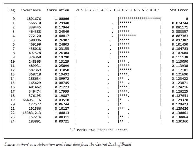
The former result warrants first order differencing. When this is done, the pattern of the ACF changed into a rapid decay towards zero, indicating that this series is stationary in differences (Figure 2).

 

FIGURE 2

Autocorrelation Function, variable IDE, level, Jan-95 to Nov-09

 

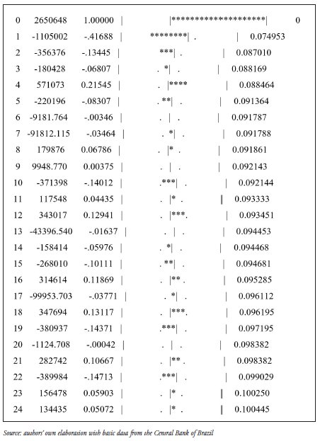
The next step was to identify the structural breaks and the corresponding outliers (Table 1).

 

TABLE 1

Outliers Search and Classification, IDE variable, January 1995 to November 2009

 

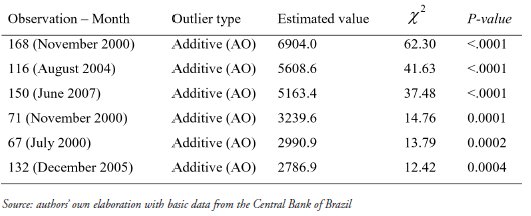
Results show that there are six outliers, all of them of the additive outlier type.

The model could then be estimated, based on the correlograms (ACF and PACF) and Cross-Correlation Functions (CCF) between each outlier and the series. Estimation required two moving average parameters of orders 1 and 12; one autoregressive parameter of order 4; and six binary intervention variables, for the following observations listed in decreasing order of t-test statistics: November 2000, August 2004, June 2007, November 2000, July 2000, and December 2005 (Table 2).

 

TABLE 2

ARIMA Models Estimates with Intervention Analysis, FDI model, Januray 1995 to November 2009

 

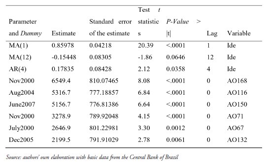
The estimate of the MA(1) parameter is statistically significant at 1% while the MA(12) is significant only at 10%. The AR(4) parameter is significant at 5%. All intervention variables are statistically significant at 1%. These results suggest a robust model (Table 2).

The MA(1) estimate shows that on average IDE errors are corrected in 85.97 units compared with the previous month; this is quite a dynamic pattern with fast correction of deviations. The MA(12) parameter shows that on average 15.44 units of the current errors are corrected vis-à-vis twelve periods earlier. Finally, the AR(4) parameter shows that 17.83 units of its current value is a function of its own value four months earlier.

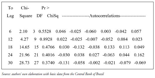
We have used the Ljung-Box test for verification of white noise pattern of residuals. Results show that the null hypothesis that all correlations are equal to zero cannot be rejected, since all p-values are above 10% (Figure 3); thus, residuals can be said to be white noise. The matrix of autocorrelations shows that all autocorrelation are of relatively small values, supporting the white noise pattern of residuals.

 

FIGURE 3

Ljung-Box (x²) test results and correlations, ARIMA model with Intervention Analysis, Variable IDE, Jan-95 to Nov-09

 

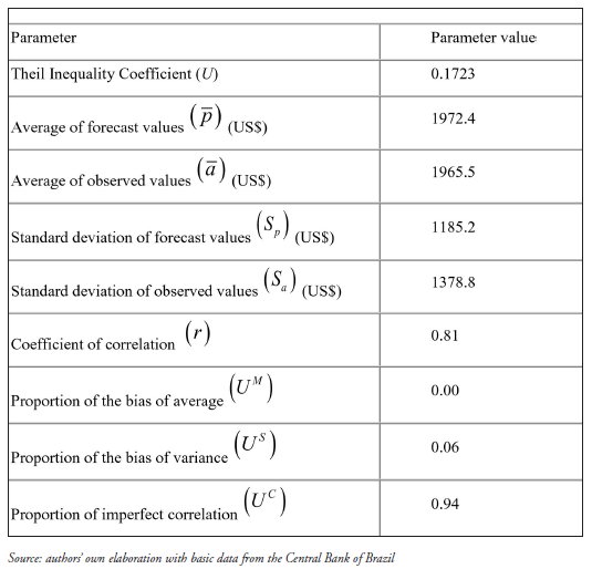
The accuracy of the forecast model was then assessed. The Theil inequality coefficient is 0.1723 – since it is closer to zero than to unity, the forecast can be viewed as satisfactory. The average of observed values (US$ 1965.5) differs only slightly from the average of forecast values (US$ 1972.4). With this small difference, the bias of average contributes with 0% to the average squared error, since its weight is only 6%. Medeiros Junior (2001) moted that according to Theil (1961, p. 37) if the ability of the predictor cannot reach perfection, the desired distribution of inequality for the three sources of errors is U^M = U^S = 0 e U^C = 1'. In this case, the proportion of imperfect correlation is the main source of squared error with 94%. On the other hand, the coefficient of correlation is 81%, showing good fit between observed and forecast values (Table 4).

 

TABLE 4

Predictive performance of ARIMA with Intervention Analysis, Variable IDE, Brazil,Jan-95 to Nov-09

 

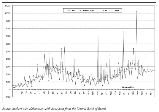
The Chart below shows the evolution of observed and forecast values for the variable IDE.

 

FIGURE 4

Variable IDE, Observed, Forecast, Maximum and Minimum Forecast Values, Jan-95 to Dec-10. Note: IDE = observed value of IDE; FORECAST = forecast value of IDE; L95 = minimum forecast value and U95 = maximum forecast value

 

FINAL REMARKS

Univariate modeling of FDI inflows into Brazil in this paper suggested quite a dynamic series with relatively rapid adjustment towards equilibrium values. The data generation process was found to show an MA(1) with coefficient 0.89. This means that errors in the variable are corrected in 89 units in relation to the previous period, suggesting that FDI is quite a dynamic economic variable that adjusts rapidly in relation to its past errors. In addition, our model showed AR(4) with a smaller coefficient of 0.17; this requires further investigation as no similar pattern was found in the literature. A previous estimate by Bashier and Talal (2007) for Jordan also found MA(1) although using annual data.

The model required intervention because the FDI series presents structural breaks or outliers. Dummy-type intervention variables were used, and the relevant observations were jul-00, nov-00, aug-04, dec-05, jun-07 and dec-08. The economic meaning of these intervention variables is mainly related to specific large operations that affect one single month, or to specific economic developments such as the economic crisis towards the end of 2008. The individual operations cannot be explained well by the theory but the bulk of the data fits well.

Although multivariate models found in the literature offer an important explanation of the movers of FDI inflows, this paper shows that univariate time series modeling contribute with relevant information to the understanding of the series dynamics. These results support the Buckley (1988) hypothesis that the pattern of the FDI series is not random or unsystematic but related to the behavior of the series over time. This means that not only are location patterns important, but there may also be a specific time-series pattern for which the best candidate is the Moving Average process. It represents a convergence in foreign direct investment inflows well, i.e., current flows should be related to past flows if an equilibrium value is still to be reached, and the errors in relation to such equilibrium are corrected relatively rapidly. The pattern of time series that was found for Brazil is also suggestive of the Uppsala, while other approaches also suggest that time patterns are relevant to the explanation of internationalization phenomena.

In light of the pattern found for the series, we have built a forecast of FDI into Brazil based on the ARIMA model we have estimated. It should be noted that forecast accuracy decreases with the number of periods forecasted. In this case, we have forecasted 13 monthly steps towards year-end 2010, and so the accuracy is significantly reduced for the more distant months forecasted. The accuracy of the forecast was measured through the Theil U-statistic as in Theil (1961, 1966), ideally close to zero, which in this case was satisfactory at 0.17.

 

REFERENCES

Bashier , A.-A. & Takal , B. (2007), «Forecasting Foreign Direct Investment Inflow in Jordan: Univariate ARIMA Model». Journal of Social Sciences 3(1), pp. 1-6.         [ Links ]

Box , G. E. P.; JENKINS, G. M. & REINSEL, G. C. (1994), Time Series Analysis: Forecasting and Control. 3^rd ed. Prentice Hall, New Jersey.         [ Links ]

Box , G.e E.P. & TIAO, G. C. (1975), «Intervention analysis with application to economic and environmental problems». Journal of the American Statistical Association, vol. 70, no. 3, Mar, pp. 70-79.         [ Links ]

Buckley , P. J. & Casson , M. C. (2003), «The future of the multinational enterprise in retrospect and in prospect». Journal of International Business Studies, 34(2), pp. 219-222.         [ Links ]

Buckley , P. J. & Casson , M. C. (1976), The Future of the Multinational Enterprise. Macmillan, London.         [ Links ]

Buckley , P. J. & Casson , M. C. (2009), «The internalization theory of the multinational enterprise: A review of the progress of a research agenda after 30 years». Journal of International Business Studies, vol. 40, pp. 1563-1580.         [ Links ]

Bucley , P. J. (1988), «The limits of explanation: testing the internalization theory of the multinational enterprise». In Journal of International Business Studies, 19(2), pp. 181-193.

Dunning , J. H. & Lundan , S. (2007), Multinational Enterprises and the Global Economy. Edward Elgar, Cheltenham.         [ Links ]

Eden , L. (2009), «Letter from the Editor-in-Chief: The JIBS40/AIB50 Anniversary Issue: Innovations in international business theory». Journal of International Business Studies, vol. 40, pp. 1407-1410.         [ Links ]

Johanson , J. & Vahlne , J.-E. (2009), «The Uppsala internationalization process model revisited: From liability of foreignness to liability of outsidership». Journal of International Business Studies, vol. 40, pp. 1411-1431.         [ Links ]

Ljung , G. M. & Box , G. E. P. (1978), «On a measure of lack of fit in time series models». Biometrika , 65, 2 (August), pp. 297-303.         [ Links ]

Medeiros-Junior , H. (2001), «Indicador antecedente para a economia carioca». Masters Dissertation, Universidade Cândido Mendes, Rio de Janeiro.         [ Links ]

Mills , T. C. (1990), Time Series Techniques for Economists. Cambridge University, New York.         [ Links ]

Theil , H. (1966), Applied Economic Forecasting. North-Holland, Amsterdam.         [ Links ]

Theil , H. (1961), Economic Forecasts and Policy. North-Holland, Amsterdam.         [ Links ]

Williamson , O. E. (1985), The Economic Institutions of Capitalism: Firms, Markets, Relational Contracting. The Free Press, New York.         [ Links ]