TOURISM: SCIENTIFIC PAPERS

Forecasting tourist in-flow in South East Asia: A case of Singapore

Previsão da afluência de turistas ao Sudeste Asiático: O caso de Singapura

Manoj Kumar¹, Seema Sharma²

 

¹Department of Management Studies, Indian Institute of Technology, New Delhi, India. E-mail: mkumar75@gmail.com

²Department of Management Studies, Indian Institute of Technology, New Delhi, India. E-mail: seemash@dms.iitd.ac.in

 

ABSTRACT

This study attempts to forecast tourist inflow in South East Asia and choses Singapore as a case. For Singapore, tourism is one of the major sources of foreign exchange earnings since it has no natural resources to support its economy. Therefore, forecasting of tourist arrivals in the country becomes very important for the reason that the forecasting may help tourism related service industries (e.g. airlines, hotels, shopping malls, transporters and catering services, etc.) to plan and prepare their resources and activities in an optimal way. In this paper, seasonal autoregressive integrated moving average (SARIMA) methodology was considered for making monthly predictions on tourist arrival in Singapore. The best model for forecasting is found out to be (1,0,1)(1,1,0)12 and monthly forecasting were obtained for two years in future. Further, various statistical tests (e.g. Dickey Fuller, KPSS, HEGY, Ljung-Box, Box-Pierce etc.) were applied on the time series for adequacy of best model to fit, residual autocorrelation analysis and for the accuracy of the prediction.

Keywords: Forecasting, Seasonal ARIMA, Tourist Arrivals, Singapore.

 

RESUMO

Este estudo tenta prever o fluxo turístico no Sudeste Asiático e escolhe Singapura como um caso. Para Singapura, o turismo é uma das principais fontes de divisas, uma vez que não possui recursos naturais para sustentar a sua economia. Portanto, a previsão de chegadas de turistas no país torna-se muito importante pelo motivo que a previsão pode ajudar as indústrias de serviços relacionados com o turismo (por exemplo, companhias aéreas, hotéis, centros comerciais, transportadoras e serviços de catering, etc.) para planear e preparar os seus recursos e atividades de uma forma otimizada. Neste trabalho, foi utilizada a metodologia SARIMA de modo a fazer previsões mensais de chegadas turísticas a Singapura. O melhor modelo de previsão é considerado ser (1,0,1) (1,1,0) 12, sendo obtidas previsões mensais num prazo de dois anos relativamente ao futuro. Além disso, vários testes estatísticos (por exemplo Dickey Fuller, KPSS, Hegy, Ljung-Box, Box-Pierce etc.) foram aplicados sobre as séries cronológicas para adequação do melhor modelo para o ajuste, da análise de auto correlação residual e para a precisão da previsão.

Palabras clave: Previsão, Seasonal ARIMA, chegadas de turistas, Singapura.

 

1. Introduction

Tourism is an activity in which a person travels to and stays in places outside his or her usual environment (e.g. hometown or city) for any number of days but less than one year. Tourism is important for any country in the world for three reasons, one, tourists travelling from foreign countries spend foreign exchange while consuming services of the host country, two, the promotion of opportunities for businesses and, three, promote interconnectedness throughout the world. While first two reasons boosts the host country's economy, the third reason offers current and future tourists the opportunities to learn about the host country, its culture and tourism services it offers.

Tourists, usually, tend to have disposable income that they are able to spend during their visits to different locations and countries. Some tourists travel for personal leisure, some for shorter vacations while other travel on official/business trips, medical tourism, sports trips or family vacations etc. In all the cases of tourism, the country being visited gets benefitted, economically and socially. According to Economic Impact Research at world Travel and Tourism Council (WTTC), the contribution of Tourism to the world economy was at 3.1% in 2013 (or US$2.2 trillion) to world gross domestic product (WGDP). World tourism also created about 101 million jobs in 2010. Employment grew by 1.8% due to an additional 1.4 million jobs that were generated by tourism activities in 2013, according to WTTC.

Amrik Singh (1997) discussed that during the decade of 1990s, the Asia Pacific region (including North East Asia, South East Asia and the Oceania) was the fastest growing tourism regions in the world. In his research, he reviewed the growth and development of the tourism industry in the Asia Pacific region and concluded that the region is expected to maintain a high rate of growth in future.

Chi and Bernard (2005) used and analyzed eight forecasting models to forecast inbound tourist arrivals to Singapore. Among the outcomes of the study, authors' remarkable conclusions were that (1) if the length of the forecast horizon is changed, the effect can be seen on the choice of the best model that fit for forecasting; and (2) a combined model could provide the best forecasting performance. On the contrast, Chi (2005) reported that the hypothesis of tourism-led economic growth is not held in the Korean economy. Author used Engle-Granger two-stage approach and a bivariate Vector Auto Regression (VAR) model to investigate the causal relations between tourism growth and economic expansion in the Korean economy. The failed hypothesis is supported by author's test of the sensitivity of causality test under different lag selections along with the optimal lag. But, do all the economies fail to show growth led by tourism?

In a study, for the 1990 to 2002 period, on relationships between tourism development and economic growth, Lee and Chang (2008) determined that tourism has greater impact on GDP in non-OECD countries compare to OECD countries (including those in Asia, Latin America and Sub-Sahara Africa). This is one of the many evidences which favors that there are some economies which see growth due to tourism. Another study, which also favors the similar conditions, is conducted in Singapore. Economic Survey of Singapore (Ministry of Trade & Industry, 2010) reported that tourism generated on average 101,200 jobs per year between 2007 and 2010 in Singapore. It also reported that tourism in Singapore was estimated at 3.5 percent (or $7.9 billion) of its economy (nominal GDP) in 2010. Earlier, Durbarry (2004) also suggested that tourism has a significant positive impact on Mauritian economic development.

Forecasting plays a major role in tourism planning. An estimate of future demand for tourism is a crucial input for the promotion of tourism projects (Cho, 2003). If the prediction of the changes in tourism demand is available, it could help greatly in developing tourism. Cho investigated the application of exponential smoothing, ARIMA, and Elman's Model of Artificial Neural Networks (ANN) time-series forecasting techniques to predict the number of international tourist arrivals in Hong Kong and concluded that ANN was the best method for forecasting.

Accuracy is particularly important when forecasting tourism demand (Witt and Witt, 1995). The author also suggested that there exists considerable scope for improving the econometric models employed in forecasting of tourism demand. The authors also argued that, although, no single forecasting method performs consistently best across different situations, yet as an alternative and worthy of considerations, researchers can focus on autoregression, exponential smoothing and econometrics models for forecasting. Lim and McAleer (2002), in their research, used Box-Jenkins Autoregressive Integrated Moving Average (ARIMA) and Seasonal Autoregressive Integrated Moving Average (SARIMA) models to forecast tourist arrivals to Australia from Hong Kong, Malaysia and Singapore. Authors also estimated mean absolute percentage error (MAPE) and root mean squared error (RMSE) to measures forecast accuracy. They concluded that, although, the ARIMA model outperforms the seasonal ARIMA models for Hong Kong and Malaysia, the forecasts of tourist arrivals are not as accurate as in the case of Singapore.

The forecasts obtained, in the study conducted by Goh and Law (2002) using models SARIMA and multivariate SARIMA (MARIMA) with intervention, were compared with other eight time series models and found that SARIMA has the highest accuracy in forecasting. Butler (1994) commented that the obvious seasonality in tourist arrival is important and it should be neglected while making forecasts for tourist arrival. Due to this important fact, various models have been developed in tourism forecasting.

In the recent research, Moss et al (2013) studied two popular time series methods, the decomposition methodology and SARIMA approach, for modeling seasonality in tourism forecasts. The two methodologies were compared and the accuracy of each of the two models was discussed. In fact, one of the best and comprehensive studies about tourism seasonality is by Baron (1975). The researcher analyzed the seasonal pattern of tourist arrivals at borders for 16 different countries over a 17 year time frame. He also commented that the seasonality in tourism is still being researched by several researchers and policy makers, all over the world.

In a competition to forecast with best model to fit, the econometric approaches for forecasting are emphasized when annual data are used whereas the time series models (such as SARIMA) usually show their advantage for higher frequency (e.g. monthly) data (Song and Li, 2008). In another study, Chen et al. (2009) compared three models of forecasting (Holt-Winters, Grey Modelling and SARIMA) to forecast inbound air traffic to Taiwan between 1996 and 2007. The authors found the SARIMA model as the best forecasting model for their time series data.

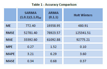
The purpose of this study is to use a popular time series method (more precisely, SARIMA) for forecasting tourist arrivals while considering the seasonality in the time series pattern of arrivals. The reason for selecting SARIMA is based upon the accuracy level obtained in this model as compare to ARIMA and Holt Winters models (Table 1). Clearly SARIMA model outperforms the other in accuracy.

 

 

The country considered for this purpose in this study is Singapore. The reasons for selecting Singapore for the study are that it is one of the most favorite destinations for tourists, the economy of Singapore is linked to the earnings from tourism and, most importantly, the accurate forecast can help in policy making, promotions and planning by government and local businesses.

 

2. Methodology

2.1 Data and procedure

The monthly tourist arrival data is from the Singapore Tourism Board (STB) and Ministry of Trade and Industry, Singapore websites [26, 27] and is available publicly. Although data were available in multi-categories, for this study purposes, we obtained the samples from STB which were specific category of international tourist arrival [27] in which STB excluded the following types of arrivals from the final dataset:

•Travelers in Singapore whose length of stay is more than one year (if stay is one year of more, then these individuals are not treated as tourists, and have a different visa types such as work permit or diplomatic etc.)

•All Malaysian citizens arriving by land (are not treated as international tourists)

•Revisiting and returning Singapore citizens, permanent residents and pass holders

•Non-resident air and sea crew (excluding sea crew flying-in to join a ship at Singapore port)

•Air transit as well as transfer passengers in Singapore (not treated as international tourists in Singapore)

The above mentioned monthly data was obtained from Singapore Tourist Board for a period January, 2003 to December, 2013.

ARIMA and SARIMA Models

Box and Jenkins (1970) are the pioneers who developed autoregressive integrated moving average (ARIMA) model for forecasting. This model still is widely used (Kumar & Anand, 2014) and many advanced forecasting models were developed keeping ARIMA as base model. The only drawbacks of ARIMA model are 1) that this model is considered for the stationary series, and 2) it is good mostly for annual data. While non-seasonal time series data can easily be used to forecast using ARIMA model, modelling of a seasonal (or high frequency) data (such as daily, weekly or monthly) requires a seasonal ARIMA model which is formed by introducing additional seasonal terms in the ARIMA model (Hyndman & Athanasopoulos, 2014). A general ARIMA model of order (p, d, q) can be expressed as follows (Pankratz, 1983):

 

 

Where, d is the order of differencing, Y_t is the most current value in data series, e_t stands for a set of uncorrected random shocks, and (1 – φ₁ B – … – φ_p B^p) is non-seasonal AR operator of order ‘p’ and (1 – φ₁ B – … – φ_q B^q) is non-seasonal MA operator of order ‘q’.

Usually, tourist arrivals often display seasonality behavior (i.e. periodic pattern) and are non-stationary time series. The seasonal ARIMA (SARIMA) model is capable of absorbing this seasonality behavior in the time series and can be written as (Pankratz, 1983):

 

 

Where B is defined as B^r Y_t = Y_{t – r}, r = s

The above process (equation 2) is a SARIMA(p,d,q)(P,D,Q)_s process, where (p,d,q) indicates the non-seasonal orders of AR, Differencing and MA terms, respectively, and (P,D,Q)_s indicate the seasonal orders of the seasonal AR, Differencing and MA terms, respectively (Chan et al, 2009). The (P,D,Q) invokes backshifts in the seasonal periods. All these parameters (p, q, d, P, D and Q) are non-negative integers.

The variable e_t is commonly referred to as white noise in time series analysis (Martinez et al, 2011) and cannot easily be explained by the model. Considering our case, the time series of monthly tourist arrivals, this white noise (e_t) can vary, for example, due to an effect of weather variables (e.g. extreme cold in the west while mild in tropical countries) or a major event (e.g. sports, formula one race etc.).

Unit Root Test and Adequacy of Models

The unit root test is used to examine whether a time series is stationary or non-stationary. When a time series is tested for unit root and result confirms the unit root in the series, the series is non-stationary. This requires unit root to be removed to transform the non-stationary series into stationary, which is obtained by differencing the series by either first order (i.e. order of differencing, d = 1) or higher order (i.e. d > 1). Care is to be taken to avoid unnecessary over differencing, which would lead to increase in the standard deviation (Kumar & Anand, 2014). The Augmented Dickey–Fuller (ADF) test (Dickey & Fuller, 1979) and Kwiatkowski-Phillips-Schmidt-Shin (KPSS) test for unit root were used in this study to test the unit root problems. The ADF test is most commonly used unit root test in forecasting (Chen et al, 2009). ADF test can be represented by following regression equation (Hyndman & Athanasopoulos, 2014):

 

 

Where, Y^'_t denotes the first-differenced series (i.e. Y^'_t = Y_t - Y_t-1), k is the number of in the regression.

In this paper, following the ARIMA model for forecasting as suggested by Box and Jenkins (Box and Jenkins, 1970), and Kumar and Anand (Kumar & Anand, 2014), seasonal ARIMA models were constructed and fitted to the tourist arrival time series data to accommodate the characteristic of seasonality as discussed earlier. The adequacy of the each model was, first, visually verified by plots of the histogram, an autocorrelation function (ACF) plot and Partial an autocorrelation function (PACF) plot of the standardized residuals, followed by the Ljung-Box test (Ljung & Box, 1978) for correlation across a specified number of time lags. To compare the goodness-of-fit of the models, the Akaike information criterion (AIC) and Bayesian information criterion (BIC) were employed. A lower AIC and/or BIC values indicate better fit of model (Burnham & Anderson, 2002).

 

3. Results and Discussions

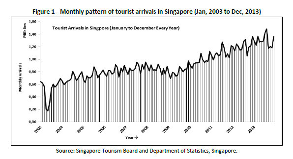
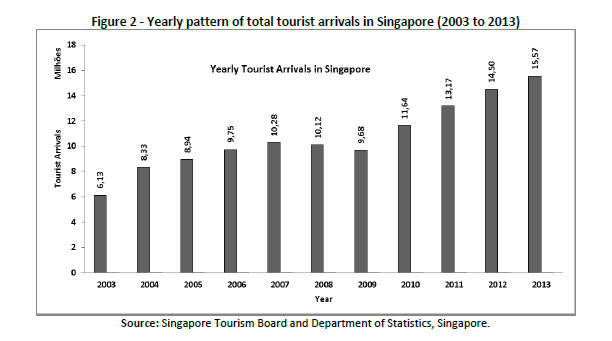
The monthly data obtained is first plotted to observe the patterns in the time series. Figure 1 and Figure 2 show the monthly and yearly tourist arrivals in Singapore. It can primarily be inferred from the figures that the time series is non-stationary with seasonality.

 

 

 

 

For better review, the time series is then decomposed to separate the three components (i.e. trend, seasonal and an irregular component) that a seasonal time series consists of. Figure 3 shows plots of these components.

 

 

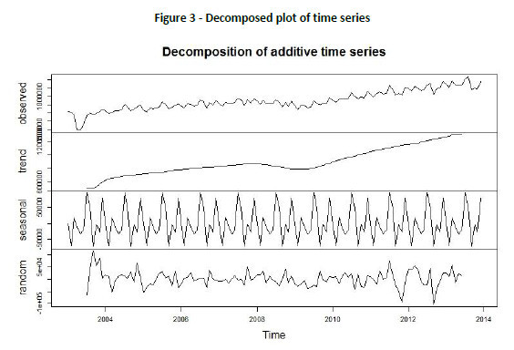
First (top) plot in Figure 3 is the original observed plot, second from top is estimated trend in the tourist arrivals, third plot from top is estimated seasonal factors and bottom plot is the estimated irregular component in the series. The estimated largest seasonal factor value is for July month (94835.48) while the lowest factor value is for January (-1592.79). One of the possible reasons for this could be the weather conditions (such as Monsoon in July). Finding these causal relations is beyond the scope of this study. Also it is observe in the estimated trend in Figure 3 that there is slight dip in tourist arrivals during 2009-10 which may be due to world financial crisis during that period. Otherwise, overall, there is an increasing trend in tourist arrivals.

Non-Seasonal Unit Root Test

We first test whether there is a unit root in the non-seasonal data (i.e. yearly data) or not. For that, we applied Augmented Dickey-Fuller (ADF) Test with three standard scenarios i.e. 1) No intercept (constant) and No Trend, 2) Intercept but No Trend; and 3) Intercept and Trend. Table 2 below shows the ADF results.

 

 

We fail to reject null hypothesis because there seems to be a unit root existence in the data, as evident from the ADF test result (in Table 2) for Case A (with no intercept and no trend) and the t-statistics (0.7758) is significantly even larger than critical value (-1.62) at 10 per cent level. Same is the result in the Case B as well (even for different lag length up to 18). But when a trend is included, Case C, we get a very different result. T-statistics we observed in this case is found to be -3.9796, which is significantly smaller than all the three critical values in the Table 1 above (i.e. critical values at 1, 5 and 10 per cent). We, therefore, failed to accept null hypothesis and infer the stationarity in the series. This result was for the highest lag difference length and remained unchanged for all other.

We then, alternatively, applied Kwiatkowski-Phillips-Schmidt-Shin (KPSS) test which has null hypothesis that the series is (level or trend) stationary whereas alternate hypothesis confirms the unit root in the series.

Following Table 3 shows the KPSS test results for various lag lengths.

 

 

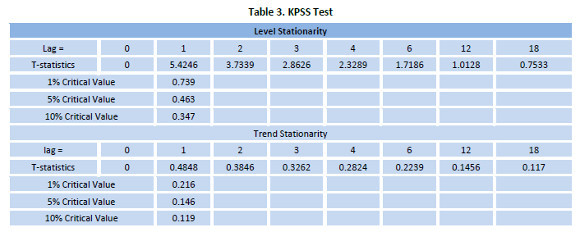
The test statistics for level and trend stationarity are larger than critical values at 5 per cent (for lag up to 12). We have no evidence that it is not trend stationary. We, therefore, fail to reject the null hypothesis at the 5 per cent level. Which means the series is not stationary in trend i.e. series has time trend with stationary errors. But for higher lags, we fail to accept the null hypothesis at 5 per cent level. Also, at 1 per cent level, we fail to accept null hypothesis because test statistics values (for trend stationarity and lag > 8) are smaller than critical values for out monthly time series data. These results are in line with the results obtained in the ADF test earlier.

Since ADF test results in Table 2 and KPSS test result in Table 3 suggests that differencing is required, first, the time series is transformed into a new logged series by taking logarithms (to the base 10) of the data exhibited in Figure 1 to induce constant variance in the series. Then this transformed series is further transformed into a differenced series of first order. The plot of this logged first differenced series is shown in Figure 4. The transformed series seems to be fluctuating about a constant mean (of 0.003) which is very close to zero mean. Therefore, the order of non-seasonal differencing can be considered to be d = 1. There is no need to go for second order differencing in the series as this process would increase the variance in the series.

 

 

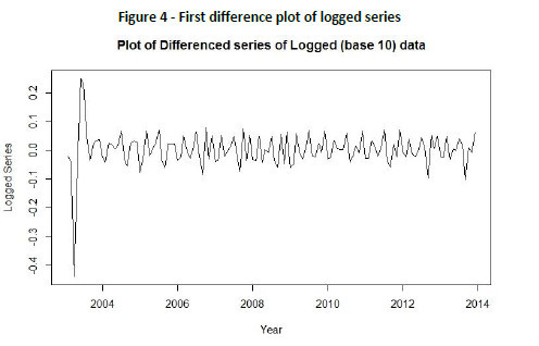
Table 4 represents the HEGY test (Hylleberg et al, 1990) results for the unit root test for transformed (first difference of logged) series. Two types of deterministic models were used, one with no intercept, no linear trend and without seasonal dummies, and another model with an intercept, a linear trend with seasonal dummies. Also, the test uses BIC methods to select lag orders to test unit root in the data (Franses, 1990, and, Beaulieu and Miron, 1993).

 

 

HEGY test statistics infer that at 5 per cent level series is stationary (both at seasonal and non-seasonal frequencies). Therefore, based on the HEGY test results above, we can confirm the values of D as 1 or first order seasonal differencing.

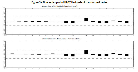
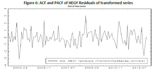
Below Figure 5 and 6 shows the residuals’ time series, auto-correlation plot (ACF) and partial auto-correlation plot (PACF) of HEGY residuals.

 

 

 

 

Further, in Figure 7 below, we show the plot of autocorrelation function (ACF) and partial autocorrelation function (PACF) of the transformed time series. It can be observed that ACF series exhibits periodicity at lag = 12 meaning a seasonal MA(1) component, confirmed by PACF as well. Also significant autocorrelation spike at lag 1 indicates a non-seasonal MA(1) component in the series.

 

 

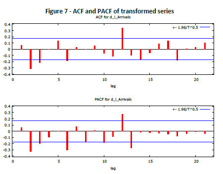
This results into an initial seasonal ARIMA(0,1,1)(0,1,1)₁₂ model with the order of differencing of 1 and seasonal and non-seasonal MA orders of Q=1 and q=1, respectively. This SARIMA model is then fitted to the time series data for further exploration. Figure 8 shows the plot, ACF and PACF of this fitted model. It is clearly evident from ACF plot that the autocorrelation spike at lag 2 and 3 are outside of significance bounds and then it slowly tails off to zero. This means there may be higher orders (p) of non-seasonal AR terms in the model. Therefore, more models needed to be considered with non-seasonal AR orders (p) of 1, 2 and 3.

 

 

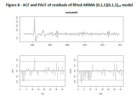
Further, from PACF plot in Figure 8, we observe that the partial autocorrelation after lag 3 tails off to zero, suggesting us that the non-seasonal AR order (p) maximum can be 3 and since at lag 1, spike is within significant bound, the minimum order can also be zero. All the suggested possible Seasonal ARIMA(p,d,q)(P,D,Q)_s models (including zero differencing order) are shown in the Table 5.

 

 

For seasonal difference order D=0, the convergence problem was faced, therefore, the ARIMA(1,0,0)(0,0,1)₁₂ model was removed from the considerations. Consequently, to select the best SARIMA model for forecasting from the above suggested models, the lowest values in errors (AIC, BIC and/or AICc) are considered. Further, Ljung-Box test be employed to test the residuals for autocorrelations.

The computed values of the mean errors (ME), root mean square errors (RMSE), mean absolute errors (MAE), mean absolute percentage errors (MAPE), mean absolute square errors (MASE), Akaike’s information criterion (AIC), Bayesian information criterion (BIC) and corrected AIC (AICc) errors (Hyndman & Athanasopoulos, 2014) for each of the suggested models are tabulated in Table 6 below.

 

 

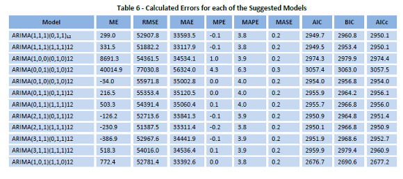
Although, in the above table that the lowest values for ME, RMSE, MAE and MPE are for different models, the lowest computed values of AIC, BIC and AICc are for the seasonal ARIMA(1,0,1)(1,1,0)₁₂ model. Therefore, we select this model as the best-fit model. The mathematical model for the seasonal ARIMA(1,0,1)(1,1,0)₁₂ can be represented by:

 

 

Following Table 7 below represents the estimated coefficients of chosen Seasonal ARIMA model:

 

 

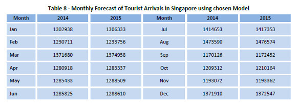
And in the Table 8 below, the monthly forecast were made for 24 months in future using the chosen model and obtained coefficients (from Table 7):

 

 

Further, to analyze the model adequacy, we will now look at residuals of the fitted model and forecast. Following Figure 9 shows the ACF, PACF and plot of residuals of the fitted model. It can easily be inferred that these are white noise and all of the residuals at various lags are well within 5 per cent significance levels. Therefore, we can assume that there are no auto-correlations existing in the residuals of that model.

 

 

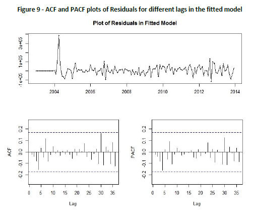
To confirm the assumption, we will apply Ljung-Box and Box-Pierce tests for independence. These test results are shown in the Table 8 below. Clearly we can infer from the large p-values of results from both tests for various lags that errors are white and are not auto-correlated.

In the above Table 8 we have shown only three results from each of the tests. A broader picture of the Ljung-Box test statistics is shown in the Figure 10 below. This figure represents the plot of p-values obtained from the Ljung-Box test for the different lags for the fitted model. Clearly, it can be confirmed that none of the p-values is equal or less than 0.05 (significance level). Hence it can be inferred that errors in the model are white and are not auto-correlated.

 

 

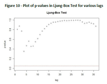
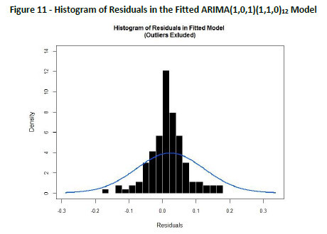
In other words, the high p-values associated with the Ljung-Box statistics confirm that we cannot reject the null hypothesis of independence in this residual series. Thus, we can say that the SARIMA (1,0,1)(1,1,0)₁₂ model fits the data well. Further, in Figure 11 (the histograms and normal distribution) and in Figure 12 (the QQ plot of normality), the error term ε_t in the fitted model clearly seems to follow normal distribution (baring one outlier as is visible in QQ plot) of the sample.

 

 

 

 

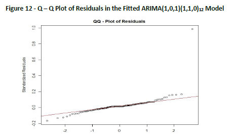
We observe in Figure 12 that except a few circles at the tails, all the circles lie quite close to the line, and hence we can say these data come from a normal distribution. These results as above are in strong support that the model chosen, i.e. ARIMA(1,0,1)(1,1,0)₁₂, can be considered as the right model to fit and the forecast values obtained using this model are strong predictions with zero auto-correlated errors.

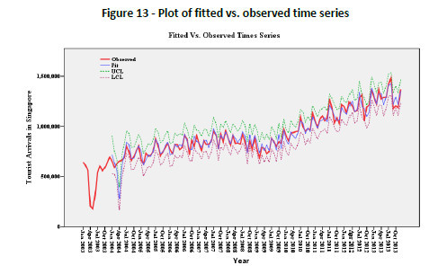
With strong evidences that the model is adequate for forecasting, we then obtain the plot of the fitted model versus observed time series. The plot is shown in the Figure 13 below. Also shown on the chart are the upper control limit (UCL) and the lower control limit (LCL) at 5 per cent level.

 

 

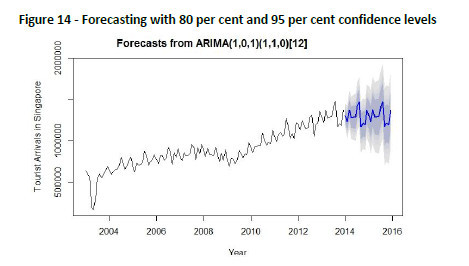
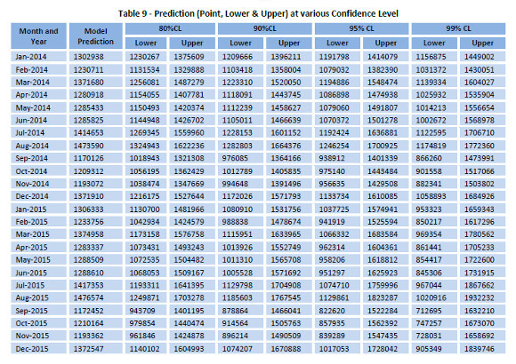
In Figure 14 we show the forecast (with 80 and 95 per cent confidence level) up to 24 months in future using the selected model and these forecast values are shown in the Table 9 below.

 

 

 

4. Conclusion

In this study, Singapore was chosen as a case for tourist inflow forecasting in South East Asia for the main reason that it does not have natural resources to support its economy and hence greatly depends upon foreign tourists not only for foreign exchange earnings but also for business exports. We collected ten years’ monthly time series data of tourist arrivals in Singapore between 2003 and 2013 from secondary sources (mainly Singapore’s government websites). The time series data was initially tested for unit root problems and further testing were done to arrive on to the best model for forecasting. Seasonal auto-regressive integrated moving average (SARIMA) methodology was adopted for forecasting (as it was found outperforming on accuracy levels as compare to the ARIMA and Holt Winters models) and the best model for fitting is found out to be of (1,0,1)(0,1,1)₁₂ order. This model was further tested for adequacy i.e. white errors (free from auto-correlation) and upon confirmation on adequacy, the model was used to make forecasting of monthly tourist inflow (arrivals) for the two years in future. The chosen model passed the major diagnostic statistical tests and showed high accuracy performance in modelling the data. The forecasts were made at various confidence levels (e.g. 80 per cent, 95 per cent etc.). This paper contributes to the literature on forecasting tourist arrivals in several ways. Firstly, the accurate model selection critical to reliable forecast to use and plan various operational activities by tourism industry businesses in Singapore. Secondly, model reliability was tested for various statistical analysis so that robustness of prediction could be obtained. Also, the forecasting errors were seen minimum as compare to other models, making it more reliable. We also attempted to provide tentative answers to some major policy questions such as what is forecast of arrival of tourists vis a vis the current trends? What will be the relative growth in arrivals in Singapore? Can the prediction be used as a tool for planning at Destination Marketing Organization (DMO) and if yes with what confidence level? Future directions of the work can me to elaborate the major impacts of forecasting with high accuracy for scholars, managers and policy makers in tourism.

According to Baggio & Klobas (2011) a Mean Absolute Percentage Error (MAPE) less than 10% shows a highly accurate forecasting performance of the model. MAPE of our model is 3.8%, yet a little improvement in forecasting accuracy could lead to large amount of savings in tourism industry. This statistically proven prediction may be used for better planning of tourism related businesses, DMOs and exporters. However there are scopes for further improvements in the forecast by using advanced techniques such as Singular Spectrum Analysis (SSA). In a recent study by Hassani et. al. (2014) found that SSA outperformed ARIMA in forecasting U.S. Tourist arrivals by country of origin. Therefore, the directions for future studies on this data can be forecasting (using models such as SSA, Vector SSA model or feed-forward Neural Network etc.) tourist arrivals from its most important foreign source markets.

 

References

Baggio, R. & Klobas, J. (2011). Quantitative Methods in Tourism: A Handbook. Aspects of Tourism Series. Bristol, Buffalo, Toronto: Channel View Publications.         [ Links ]

Bar On, R. R. (1975). Seasonality in Tourism: A Guide to the Analysis of Seasonality and Trends for Policy Making. Vol. 2, London: The Economist Intelligence Unit Ltd.         [ Links ]

Joseph, B. J. & Miron, J. A. (1993). Seasonal Unit Roots in Aggregate U.S. Data. Journal of Econometrics, 55(1-2), 305-328.         [ Links ]

Box, G. E. P. and Jenkins, G. M. (1970). Time series analysis: Forecasting and control, San Francisco: Holden-Day.         [ Links ]

Burnham K. P. & Anderson D. R. (2002). Model Selection and Multimodel Inference: A Practical Information-Theoretic Approach. 2^nd Edition, New York: Springer        [ Links ]

Butler, R. W. (1994). Seasonality in Tourism: Issues and Problems. In Seaton et al (edition) Tourism: the State of the Art. Chichester: Wiley & Sons.         [ Links ]

Chen, C. F., Chang, Y. H., & Chang, Y. W. (2009). Seasonal ARIMA forecasting of Inbound Air Travel Arrivals to Taiwan. Transportmetrica, 5(2), 125-140.         [ Links ]

Cho, V. (2003). A Comparison of Three Different Approaches to Tourist Arrival Forecasting. Tourism Management, 24(3), 323-330.         [ Links ]

Dickey, D. A. & Fuller, W. A. (1979). Distribution of the Estimators for Autoregressive Time Series with a Unit Root. Journal of the American Statistical Association, 74 (366), 427-431.         [ Links ]

Durbarry, R. (2004). Tourism and Economic Growth: The Case of Mauritius. Tourism Economics, 10(4), 389-401.         [ Links ]

Franses, P. H. (1990). Testing for Seasonal Unit Roots in Monthly Data. Technical Report No. 9032. Rotterdam: Econometric Institute, Erasmus University.         [ Links ]

Goh, C. and Law, R. (2002). Modeling and Forecasting Tourism Demand for Arrivals with Stochastic Nonstationary Seasonality and Intervention. Tourism Management, 23(5), 499-510.         [ Links ]

Hylleberg, S., Engle, R. F., Granger, C. W. J. & Yoo, B. S. (1990). Seasonal Integration and Co-integration. Journal of Econometrics, 44, 215-238.         [ Links ]

Hyndman, R. J. & Athanasopoulos, G. (2014). Forecasting: Principles and Practice. Retrieved March 4, 2014 from https://www.otexts.org/fpp/        [ Links ]

Kumar, M. & Anand, M. (2014). An Application of Time Series ARIMA Forecasting Model for Predicting Sugarcane Production in India. Studies in Business and Economics, 9(1), 81-94.         [ Links ]

Lee, C. C. & Chang, C. P. (2008). Tourism Development and Economic Growth: A Closer Look at Panels. Tourism Management, 29(1), 180–192.         [ Links ]

Lim, C. & McAleer, M. (2002). Time Series Forecasts of International Travel Demand for Australia. Tourism Management, 23(4), 389-396.         [ Links ]

Ljung, G. M. & Box, G. E. P. (1978). On a Measure of Lack of Fit in Time Series Models. Biometrika, 65, 297-303.         [ Links ]

Martinez, E. Z., Soares da Silva, E. A. & Fabbro, A. L. D. (2011). A SARIMA Forecasting Model to Predict the Number of Cases of Dengue in Campinas, State of São Paulo, Brazil. Revista da Sociedade Brasileira de Medicina Tropical, 44(4), 436-440.         [ Links ]

Oh, C.O., (2005). “The Contribution of Tourism Development to Economic Growth in the Korean Economy”. Tourism Management, 26(1), 39-44.         [ Links ]

Oh, C.O. and Morzuch, B.J. (2005). Evaluating Time-series Models to Forecast the Demand for Tourism in Singapore: Comparing Within-sample and Post-sample Results. Journal of Travel Research, 43(4), 404-413.         [ Links ]

Pankratz, Alan (1983). Forecasting with Univariate Box - Jenkins Models: Concepts and Cases. New York: John Wiley & Sons.         [ Links ]

Singh, Amrik (1997). Asia Pacific Tourism Industry: Current Trends and Future Outlook. Asia Pacific Journal of Tourism Research, 2(1), 89-99.         [ Links ]

Singh, Amrik (2000). The Asia Pacific Cruise Line Industry: Current Trends, Opportunities and Future Outlook. Tourism Recreation Research, 25(2), 49-61.         [ Links ]

Song, H. and Li, G. (2008). Tourism Demand Modelling and Forecasting – A Review of Recent Research. Tourism Management, 29(2), 203-220.         [ Links ]

Witt, S.F. and Witt, C.A. (1995). Forecasting Tourism Demand: A Review of Empirical Research. International Journal of Forecasting, 11(3), 447–475.         [ Links ]

Singapore Tourism Board: Data on tourists. Retrieved March 4, 2014 from https://www.stb.gov.sg/statistics-and-market-insights/Pages/statistics-Visitor-Arrivals.aspx.         [ Links ]

Ministry of Trade and Industry, Singapore. Retrieved March 4, 2014 from http://www.mti.gov.sg/        [ Links ]

World Travel and Tourism Council. Retrieved March 4, 2014 from http://www.wttc.org/.         [ Links ]

Hassani, H., Webster, A., Silva, E. S., & Heravi, S. (2015). Forecasting US tourist arrivals using optimal singular spectrum analysis. Tourism Management, 46, 322-335.         [ Links ]

 

Article history:

Submitted: 28.09.2014

Received in revised form: 07.12.2015

Accepted: 07.12.2015