


Serviços Personalizados
Journal
Artigo
 Inglês (pdf)
 Artigo em XML
 Referências do artigo
 Enviar este artigo por email
Indicadores
-
 Citado por SciELO
 -
 Acessos
Links relacionados
-
 Similares em
SciELO
Similares em
SciELO
Compartilhar

 Permalink
Corrosão e Protecção de Materiais
versão On-line ISSN 2182-6587
Corros. Prot. Mater. vol.34 no.2 Lisboa dez. 2015
ARTIGO
Atmospheric corrosion of mild steel in marine atmospheres
Corrosão atmosférica do aço macio em atmosferas marinhas
E. Pino(1), J. Alcántara(1), B. Chico(1), I. Díaz(1), J. Simancas(1), D. de la Fuente(1) and M. Morcillo(1)(*)
(1) National Centre for Metallurgical Research (CENIM/CSIC), Department of Surface Engineering Corrosion and Durability, Avda. Gregorio del Amo, 8, 28040 – Madrid, Spain E-mails: epinodirauso@gmail.com; jenialcantara@hotmail.com; bchico@cenim.csic.es; ivan.diaz@cenim.csic.es; jsimancas@cenim.csic.es; delafuente@cenim.csic.es
(*) Corresponding author: morcillo@cenim.csic.es
ABSTRACT
Research has been carried out for 6 months in seven pure marine atmospheres with average chloride deposition rates (salinities) of 41-886 mg Cl-/m2.day. The paper considers the entrainment of marine aerosol inland and the exponential relationship between the atmospheric salinity values and the shore distance. The paper also considers mild steel corrosion rate and the resulting corrosion products and layers, and its dependence of atmospheric salinity of the site. Characterization of corrosion products was performed by SEM and XRD. In addition to lepidocrocite and goethite (major contents), high akaganeite and magnetite (minor contents) were found in the corrosion products, the latter ones found mainly at the steel/rust interface.
Key-words: Mild Steel, Corrosion, Marine Atmospheres, SEM, XRD
RESUMO
Foi realizada uma investigação durante seis meses em sete atmosferas marinhas com velocidades de deposição de cloretos (salinidades) médias compreendidas entre 41 e 886 mg Cl-/m2.dia. O presente trabalho considera a influência do avanço do aerosol marinho e a variação exponencial entre os valores da salinidade atmosférica e a distância à costa. Apresenta também a velocidade de corrosão do aço macio e os produtos e camadas de corrosão resultantes e a sua dependência da salinidade atmosférica local. A caracterização dos produtos de corrosão foi realizada por microscopia electronica de varrimento (MEV) e difracção de raios X (DRX). Para além da lepidocrocite e goetite (maiores teores), foram ainda encontradas akaganeite e magnetite (menores teores), principalmente na interface aço/ferrugem.
Palavras Chave: Corrosão, Aço Macio, Atmosferas Marinhas, MEV, DRX
1. INTRODUCTION
The atmospheric corrosion of metals is an electrochemical process which is the sum of individual processes that take place when an electrolyte layer forms on the metal. This electrolyte can be either an extremely thin moisture film (just a few monolayers) or an aqueous film of hundreds of microns in thickness (when the metal is perceptibly wet). Aqueous precipitation (rain, fog, etc.) and humidity condensation due to temperature changes (dew) are the main promoters of metallic corrosion in the atmosphere.
The magnitude of the corrosion fundamentally depends upon the length of time that the surface is wet, although it is, in fact, a function of a series of factors, such as rain, relative humidity, temperature, exposure conditions, atmospheric pollution, composition of the metal, properties of the formed oxide, etc.
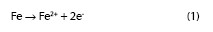
Atmospheric corrosion, as a global process, includes simultaneous oxidation and reduction reactions. The anodic reaction, consisting of the oxidation of the metal, can be given as:
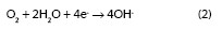
The reduction of oxygen in neutral or basic media takes place according to the reaction:
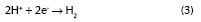
Only in the case of a high degree of pollution with acid products does the cathodic reaction of a discharge of hydrogen ions becomes of importance
Atmospheric salinity in coastal regions notably increases the atmospheric corrosion rate of steel in comparison with a clean atmosphere, as marine chlorides dissolved in the moisture layer considerably raise the conductivity of the electrolyte film on the metal and tend to destroy any passivating films. The corrosion rate is a function of the chloride deposition rate (1).
In general, atmospheric corrosion studies consider very few test sites located in marine atmospheres, often with not particularly high Cl-ion deposition rates and frequently affected by SO2 pollution. In the present work research has been carried out at 7 testing stations located at distances of between 332 m and 2,500 m from the shoreline, allowing the study of steel corrosion across a broad spectrum of atmospheric salinities in pure marine atmospheres (without significant SO2 pollution). This paper assesses the mild steel corrosion rate and analyses the resulting corrosion products and layers, and its dependence of atmospheric salinity of the site of exposure.
2. EXPERIMENTAL
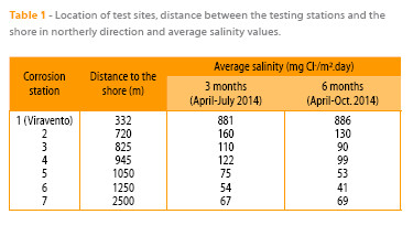
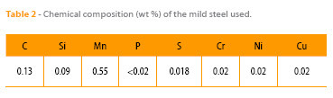
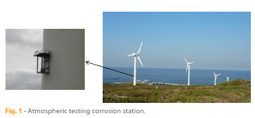
Research has been carried out in the pure marine atmosphere at Cabo Vilano wind farm (Camariñas, Spain) at seven corrosion stations located at different distances from the shoreline (Table 1). Meteorological data were supplied by a weather station belonging to the Spanish Meteorological Agency (AEMET), situated very close (25 m) to corrosion station 1 of Viravento. The seven atmospheric corrosion stations were equipped with the necessary instrumentation to measure atmospheric pollution in terms of SO2 (2, 3) and Cl– (4). The atmospheric SO2 content was negligible (0.96-1.44 mg SO2/m2.day) (5). Panels of mild steel (whose composition is shown in Table 2) measuring (100 x 50 x 2) mm were exposed in quadruplicate for 3 and 6 months (April-September 2014) on open-air racks at an angle of 90° from the horizontal plane at the seven test sites. After 3 and 6 months of exposure the specimens were withdrawn from the testing stations in order to obtain data on mass loss due to corrosion (in triplicate) and a fourth specimen was employed for characterisation of the corrosion products formed. Each station (Fig. 1) was fixed by magnets to the leg of a wind turbine, facing north, which according to historic records is a dominant wind direction at the exposure site. The station consisted of a rack holding the atmospheric salinity measuring device (wet candle (4)) at the bottom and the mild steel specimens at the top.
The corrosion rate of the steels during atmospheric exposure was determined gravimetrically by mass loss using a solution of hydrochloric acid and hexamethylenetetramine (corrosion inhibitor) according to ISO 8407, Annex A, designation C.3.5 (6). In all cases a Mettler AT261 DeltaRange microbalance to the nearest 10-4 g was used.
From visual observation of the rusts formed in the atmosphere it is possible to identify different types of morphology: powdery rust particles, grains, flakes and sheets or laminations that peel off easily (7). In severe marine atmospheres, as is the case of station 1, in conditions with a high chloride content and long moisture retention times, it is common to see the formation of coarse flakes and layered sheets. The exposure of carbon steel in these atmospheres can lead to the formation of thick rust layers containing a number of “compact laminas”. These thick rust layers tend to become detached from the steel substrate, leaving it uncovered and without protection, and thus accelerating the metallic corrosion process (7). With the assistance of a very thin sharp blade, those compact laminas were carefully separated from the exfoliated rust layer to be analysed separately.
XRD analysis was carried out on powdered rust samples obtained by grinding in an agate mortar the corrosion product layer formed on the skyward surface of the steel specimens, screening the rust to obtain a particle size of less than 125 μm. XRD measurements were performed with a Bruker AXS D8 diffractometer equipped with a Co X-ray tube, goebel mirror optics and a LynxEye Linear Position Sensitive Detector for ultra-fast XRD measurements. This type of radiation is especially suitable for iron-rich samples to avoid the strong fluorescence resulting from copper radiation and to produce high resolution data. A current of 30 mA and a voltage of 40 kV were employed as tube settings. Operating conditions were selected to obtain XRD profiles of sufficient quality, namely optimal counting statistics, narrow peaks, and detection of small diffraction peaks of minor phases. The XRD data was collected over a 2θ range of 10-80° with a step size of 0.02°. The qualitative identification of crystalline phases present in the rust formed on steels was performed from XRD patterns using the JCPDS database and DIFFRACplus EVA software by Bruker AXS.
Microscopic observation of the rust layers formed has been carried out using a Nikon model Epiphot 300 polarised light optical microscope equipped with an Infinity 2 camera, and a Hitachi S4800 high resolution scanning electron microscope (SEM) (3 nm in high vacuum mode) equipped with secondary electron and backscattered electron detectors and an Oxford Inca energy dispersive microanalysis system (EDS). Microscopic analysis was carried out on cross sections, observing the structure of the rust layer and on the metal surface, observing the morphology of the different corrosion products comprising the rust.
3. RESULTS AND DISCUSSION
The area of Cabo Vilano wind farm presented during the exposure time a high relative humidity (RH 86.8 %) and mild temperature (Tavgavg 16.3 °C), together with high precipitation rates. These values indicate high times of wetness of the metallic surface which favour atmospheric corrosion processes.
3.1. Entrainment of marine aerosol inland
Aerosol particles can be entrained inland by marine winds, settling after a certain time and after travelling a certain distance. The wind regime directly influences aerosol production and transportation, and is significantly affected by geostrophic winds, large-scale atmospheric stability, and the difference between diurnally-averaged land and sea temperatures, which varies according to the season of the year. It is also dependent on the latitude, ruggedness of the coastline, and undulation of the land surface (8, 9). A reduction in the size and mass of aerosol particles due to drying of the droplets can considerably increase the entrainment distance.
The largest fraction (by mass) of aerosol particles have diameters of between 8 μm and 80 μm (8). The largest aerosol particles (diameter > 10 μm) remain in the atmosphere for short time periods; the larger the particle size the shorter the time. In contrast, particles of a diameter of < 10 μm can travel hundreds of kilometres in the air without settling (10).
It is known that the main effect of marine atmospheres reaches just a few hundreds of metres from the shoreline and subsequently drops off further inland (10). This initial decrease in the marine aerosol particle concentration (atmospheric salinity) is due mainly to a dry deposition process. Essentially two mechanisms are responsible for the dry deposition of aerosol (11): (a) sedimentation due to the effect of gravity, and (b) removal by contact of the turbulent air mass with the land. This effect depends on the roughness and type of terrain (open land, presence of vegetation, etc.).
Thus, the possibility of aerosol particles reaching points that are more or less distant from the shoreline will depend on the balance between entrainment inland by the action of marine winds and deposition on the land by the aforementioned mechanisms. This matter was addressed in previous studies (1, 12) by developing a simple exponential model of the variation in atmospheric salinity with distance from the shore.
In the present study an exponential relationship is also clearly seen between the atmospheric salinity values obtained in the three-monthly periods from April 2014 to June 2014 and July 2014 to September 2014 and the distance between stations 1 to 7 and the shoreline (Fig. 2). The corresponding exponential equations would be:
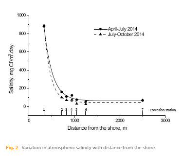
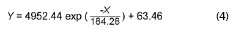
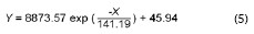
being Y the atmospheric salinity expressed as mg Cl-/m2.day and X the distance from the shore in meters (m).
3.2 Mild steel marine atmospheric corrosion and its dependence of atmospheric salinity
3.2.1 Corrosion versus atmospheric salinity
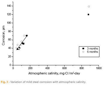
In studies of atmospheric corrosion in marine atmospheres, a direct relationship is generally established between corrosion and the saline content of the atmosphere. Ambler and Bain (10) were the first to demonstrate this relationship, which has subsequently been addressed in many other papers, such as the work of M. Morcillo et al. presenting abundant bibliographic information for atmospheric salinities of up to 600 mg Cl-/m2.day (13) and of Alcántara et al. who extended the atmospheric salinity range to values in excess of 600 mg Cl-/m2.day (1).
Figure 3 has been elaborated with data obtained in this study. For atmospheric salinities less than 200 mg Cl-/m2.day a linear relationship between corrosion of steel and salinity is clearly established. The lack of data between 200 and 900 mg Cl-/m2.day (only one point corresponding to the station 1) prevents to draft any conclusion, however can be inferred that for salinities well above 200 mg Cl-/m2.day steel corrosion seems to be stabilized.
3.2.2 Rust phases formed and its evolution with time of exposure
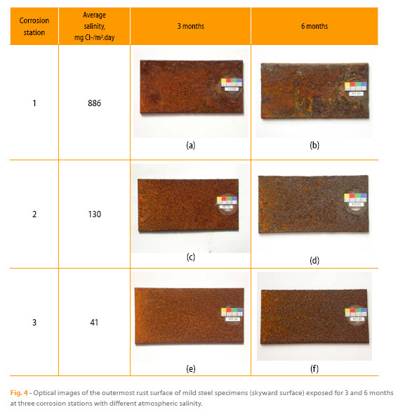
The surface appearance (Figure 4) of the patinas formed after 3 and 6 months of exposure in corrosion stations 1, 2 and 6, with very different atmospheric salinities, varies according to the aggressiveness of the environment. Thus a lighter colored rust is observed in the less aggressive station 6 (Figure 4e) while darker patinas are seen in the most aggressive atmosphere (station 1, Figure 4a). Patinas are darker with time of exposure. With regard to texture, smoother rusts (more homogeneous and finer granulometry) are observed in the less aggressive atmosphere (station 6, Figure 4e) whereas the rust textures are rougher, their appearance more heterogeneous and their grain sizes coarser in the more aggressive atmosphere of station 1 (Figure 4a). In station 1 (Figure 4 a-b ) exfoliations of the rust layers are observed.
The corrosion products most commonly found in rust formed on steel exposed at the atmosphere are lepidocrocite (g-FeOOH), goethite (a-FeOOH) and magnetite (Fe3O4) /maghemite (g-Fe3O4). Hiller (14) considers that lepidocrocite is the first crystalline corrosion product to form. In mild acid solutions lepidocrocite is transformed into goethite, which is the most stable of the different oxyhydroxides. Magnetite is also one of the main constituents of rust and is usually detected in the inner zone closest to the base steel, where the oxygen concentration is Salinity, mg Cl-/m2.day depleted. In marine atmospheres, where the surface electrolyte contains Corrosion, µm chloride, akaganeite (b-FeOOH) also forms (15) and magnetite contentis usually higher (14). Other phases (feroxyhyte (d-FeOOH), ferrihydrite (FeHO.4HO), hematite (a-FeO), etc.) can also be formed.
When semi-quantitative XRD information about the content of the different phases in the rust is required, the quickest way to carry out XRD analysis is to use the reference intensity ratio (RIR) method. Semiquantitative analysis was thus performed using the I/Ic ratio from each phase (where I is the intensity of the strongest peak of the phase and Ic is the intensity of the strongest corundum reflection in a 50/50 weight fraction mixture) taken from the Powder Diffraction Files (PDF) card (16).
However, the RIR method is subject to high inaccuracy in this case due to systematic peak overlap of the different phases present. This problem can be overcome by using Rietveld analysis. As this method fits the whole diffraction pattern, all reflections, overlapping or not, are used in the fitting process, and the complex severely overlapped patterns of our samples can, in principle, be analysed. For this reason, the Rietveld method has been widely reported as one of the most suitable techniques for quantifying crystalline phases in multiphase systems from the XRD pattern (17, 18). In this work, version 4.2 of the TOPAS Rietveld analysis program (Bruker AXS) was used for XRD data refinement. For the application of Rietveld refinement, instrument functions were empirically parameterised from profile shape analysis of a corundum sample measured in the same conditions. The refinement protocol also included the major parameters like background, zero displacement, scale factors, peak breadth and unit cell parameter. The quality and reliability of the Rietveld analysis was quantified by the corresponding figures of merit: the weighted sum of residuals of the least squares fit, R, the statitiscally expected least squares fit, R, the wpexpprofile residual, Rp, and the goodness of fit (sometimes referred as chi-squared), GF.46 Since gF = R /R, a gF = 1.0 means a perfect fitting.
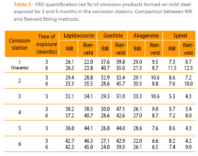
Table 3 sets out the corresponding quantifications of the different rust phases found making a comparison between the two fitting methods, RIR and Rietveld. The three iron oxyhydroxides, lepidocrocite, goethite and akaganeite, were identified in all the samples, along with the strongest diffraction peak corresponding to a cubic iron oxide, magnetite and/or maghemite. Because both oxide compounds crystallise in a spinel crystal structure and their lattice parameters are very similar, their diffractograms are practically identical. Both phases are associated to the diffraction angle next to 35° (19). As it is very complicated to discriminate between magnetite and maghemite, both being cubic iron oxides, have been referred to in this paper as “spinel”. As can be deduced from Table 3, the RIR method underestimates very notably the goethite phase content and overestimates the akaganeite (very notably) and spinel (slightly) phase contents. In rust phase mixtures containing akaganeite and spinel, as in this study, the most intense spinel peak (113), at ~ 35.4° for Cu radiation, overlaps with several akaganeite reflections, producing a high relative error in the determination of both phase fractions with the RIR method. Use of the RIR method also provides only low accuracy in the quantification of goethite because it does not include any correction to quantify the texture effect. Orientation problems can also be recognised when using Rietveld refinement and then corrected by the introduction of preferred orientation modelling parameters for goethite on the crystallographic plane (101) according to the March-Dollase model (20).
The high atmospheric salinities recorded throughout the entire exposure time and high times of wetness have created suitable conditions for the formation of akaganeite in all corrosion stations. This has not been the case in many field studies reported in the literature that have failed to identify the akaganeite phase among the corrosion products formed, even in marine atmospheres with important Cl- ion deposition rates (5), raising uncertainty as to what conditions are necessary for the formation of this oxyhydroxide. To elucidate this point the authors have been carrying out a study to clarify the environmental conditions that lead to the formation of akaganeite: an average RH around 80 % or higher and simultaneously an average chloride deposition rate of around 60 mg/m2.day or higher (5), both conditions generally fulfilled in the study presented in this paper. It is interesting to know the variation of rust phases content with the salinity of the site. Looking at Figure 5 can be observed that as atmospheric salinity increases the akaganeite, goethite and spinel contents are higher, 43.9 %, 39.4 % and 107.1 % respectively, particularly in the latter rust phase. In contrast, the lepidocrocite content is notably lower (52.5 %). Tamaura et al. (21) suggest that lepidocrocite is transformed into spinel in the absence of oxygen according to the reaction:
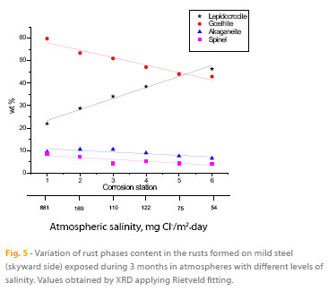
It is important to observe how the different rust phase contents vary when the exposure time increases from 3 to 6 months (stations 1, 2, 4 and 6 in Table 3). The values obtained, after applying the Rietveld fitting method, show no great variations in the lepidocrocite, goethite and akaganeite contents but a considerable increase in the spinel phase content. This seems to indicate a gradual spinel-enrichment of the steel/rust interface as a consequence of electrochemical reduction of the iron oxyhydroxides (22, 23). The fact that no clear decrease in the content of these oxyhydroxides is seen with exposure time may be due to their ongoing formation as a consequence of prolonged exposure to the atmosphere.
4. CONCLUSIONS
The following are the most relevant conclusions of this work:
- Both atmospheric salinity and the steel corrosion obey an experimental decay function with the distance from the shore.
- For atmospheric salinities less than 200 mg Cl-/m2.day a linear relationship between corrosion of mild steel and salinity is clearly established.
- For XRD quantification of rust phases formed on mild steel exposed in marine atmospheres it is necessary to carry out fitting of the diffraction pattern using the Rietveld method. The semi- quantitative analysis performed by the Reference Intensity Ratio (RIR) method is subject to high inaccuracy due to systematic peak overlaps of the different rust phases.
- As atmospheric salinity increases, goethite, akaganeite and spinel contents are higher. In contrast, lepidocrocite content is notably lower.
- As atmospheric salinity increases, corrosion layers are less compact, more cracked and even can exfoliate from the underlying steel.
- The SEM morphology of the different rust phases formed varies considerably. On the outermost surface of the rust lepidocrocite and goethite are more abundant. On the contrary, on the residual base steel from which the exfoliated rust layer was detached (very severe marine atmosphere), the formation of magnetite and akaganeite was predominant.
REFERENCES
(1) J. Alcántara, B. Chico, I. Díaz, D. de la Fuente and M. Morcillo, Corros. Sci., 97, 74-88 (2015). [ Links ]
(2) g. R. Carmichael, Report on Passive Samplers for Atmospheric Chemistry Measurements and their Role in gaw, World Meteorological Organization, geneve (1997).
(3) Air Quality Monitoring-diffusive and passive sampling (cited July 3th 2011), http://www.diffusivesampling.ivl.se
(4) EN ISO 9225: 2012. (Corrosion of metals and alloys - Corrosivity of atmospheres - Measurement of environmental parameters affecting corrosivity of atmospheres), European Committee for Standardization, Brussels (2012).
(5) M. Morcillo, J. M. González-Calbet, J. A. Jiménez, I. Díaz, J. Alcántara, B. Chico, A. Mazarío-Fernández, A. Gómez-Herrero, I. Llorente and D. de la Fuente, Corrosion (in press) (2015). doi: 10.5006/1672 [ Links ]
(6) ISO 8407: 1991. (Corrosion of metals and alloys - Removal of corrosion products from corrosion test specimens), International Organization for Standardization, genève (1991).
(7) B. Chico, J. Alcántara, E. Pino, I. Díaz, J. Simancas, A. Torres-Pardo, D. De la Fuente, J. A. Jiménez, J. F. Marco, J. M. gonzález-Calbet and M. Morcillo, Corros. Rev (in press), (2015).
(8) D. C. Blanchard and A. H. Woodcock, Ann. NY Acad. Sci., 338, 330-347 (1980). [ Links ]
(9) J. W. Fitzgerald, Atmos. Environ., 25A, 533-545 (1991). [ Links ]
(10) H. R. Ambler and A. A. J. Bain, J. Appl. Chem., 5, 437-527 (1955). [ Links ]
(11) T. A. McMahon and P.J. Denison, Atmos. Environ., 13, 571-585 (1979). [ Links ]
(12) S. Feliu, M. Morcillo and B. Chico, Corrosion, 55, 883-891 (1999). [ Links ]
(13) M. Morcillo, B. Chico, E. Otero and L. Mariaca, Mater. Perform., 38, 72-77 (1999). [ Links ]
(14) J. E. Hiller, Werkst. Korros., 17, 943-951 (1966). [ Links ]
(15) P. Keller, Werkst. Korros., 20, 102-108 (1969). [ Links ]
(16) C. R. Hubbard and R.L. Snyder, Powder Diffr., 3, 74-77 (1988). [ Links ]
(17) H. M. Rietveld, J. Appl. Crystallogr, 2, 65-71 (1969). [ Links ]
(18) D. L. Bish and S. A. Howard, J. Appl. Crystallogr, 21, 86-91 (1988). [ Links ]
(19) L. Lutterotti and P. Scardi, J. Appl. Crystallogr, 23, 246-252 (1990). [ Links ]
(20) W. A. Dollase, J. Appl. Cryst., 19, 267-272 (1986). [ Links ]
(21) Y. Tamaura, K. Ito and T. Katsura, J. Chem. Soc., Dalton Trans., 2, 189-194 (1983). [ Links ]
(22) T. Nishimura, H. Katayama, K. Noda and T. Kodama, Corrosion, 56, 935941 (2000). [ Links ]
(23) V. Lair, H. Antony, L. Legrand and A. Chaussé, Corros. Sci., 48, 2050-2063 (2006). [ Links ]
(24) K. Ståhl, K. Nielsen, J. Jiang, B. Lebech, J. C. Hanson, P. Norby and J. van Lanschot, Corros. Sci., 45, 2563-2575 (2003). [ Links ]
(25) A. Raman, S. Nasrazadani and L. Sharma, Metallography, 22, 79-96 (1989). [ Links ]
(26) A. Razvan and A. Raman, Pract. Met, 23, 223-236 (1986). [ Links ]
(27) A. Raman, S. Nasrazadani, L. Sharma and A. Razvan, Pract. Met, 24, 535548 (1987). [ Links ]
(28) A. Raman, S. Nasrazadani, L. Sharma and A. Razvan, Pract. Met, 24, 577589 (1987). [ Links ]
(29) T. Ishikawa, Y. Kondo, A. Yasukawa and K. Kandori, Corros. Sci., 40, 12391251 (1998). [ Links ]
ACKNOWLEDGEMENTS
The authors gratefully acknowledge the financial support for this study from the Ministry of Science and Innovation of Spain (CICYT-MAT 2008-06649). The authors would like to express their gratitude to the companies ENEL and gAS NATURAL for the facilities provided and for allowing the location of the corrosion stations at Cabo Vilano wind farm (Camariñas, Spain). A special acknowledgement must be done to Dr. J. A Jiménez for interpretation of XRD measurements. E. Pino acknowledges the scholarship financed by Universidad Simón Bolívar (Caracas, Venezuela) to carry out this project in CENIM/CSIC. I. Díaz also acknowledges the PhD scholarship financed by CSIC JAE Programme.

