Chemical Speciation and Dissolved Iron in the Pore Water of Patos Lagoon Sediments - Brazil

 

S.E.T. Wotter^1,*, L.F.H. Niencheski² and M.R. Milani¹

¹Escola de Química e Alimentos - FURG, Av. Itália, km 8, Rio Grande-RS, Brazil

²Instituto de Oceanografia - FURG, Av. Itália, km 8, Rio Grande-RS, Brazil

 

Abstract

Sediments can sink or deliver elements to water column. Iron is considered an essential element for the development of cyanobacteria and a limitant to phytoplankton growth. Studies on the chemical speciation of iron in seawater have been conducted, but there is no information about its chemical speciation in pore water, as reported here. This paper presents a voltammetric method to analyze dissolved iron and its chemical speciation in sediment pore water, using adsorptive cathodic stripping voltammetry (AdCSV) and the technique of competitive ligand exchange (CLE-AdCSV), respectively. The limit of detection (LOD = 0.30×10^-6 mol L^-1), the quantification (LOQ = 0.90×10^-6 mol L^-1), precision (RSD = 4.9%) and accuracy (98%), were calculated from experiments using certified reference material SLRS-4 (National Research Council Canada). The chemical speciation of pore water from sediment samples collected during April 2009, in the Patos Lagoon Estuary (RS, Brazil), was analyzed for the first time, revealing that the ratio (labile iron to dissolved iron) is significantly lower in pore water extracted from sediments of the upper layer (0 to -5 cm), than from the overlaying water or of the pore water extracted from sediments of the lower layer (-15 to -20 cm).

Keywords: iron, speciation, sediments, pore water, voltammetry.

 

Introduction

The presence of metals in the environment may threat the biota, especially if they are not naturally degraded and are bioaccumulated by plants and animals. The presence of dissolved metals in the water column is of particular concern because of their high mobility and bioavailability to aquatic organisms. The metals present in the sediment may characterize a situation of persistent contamination for long periods [1], which can be distributed between the liquid phase (including the pore water and overlying water) and the solid phase (including the sediment and solid suspended materials). The sediment plays an important role, particularly in the flow of metals in estuarine systems, and can serve as a source or sink of these elements to the water column [2].

Biogeochemical processes control the partitioning and cycling of metals between these compartments and have significant implications in the regulation of exchanges between sediment and water. The cycling occurs predominantly near the interface water/sediment, where the metal concentrations in pore water are typically higher than in deeper layers, resulting in flows of dissolved metals toward the water column, and its subsequent enrichment. Studies of metal chemical speciation in natural waters can provide information to predict their geochemical behavior, as well as their bioavailability, because the metal labile fraction is determined. In coastal regions of high activity reaction, due to changing environmental conditions such as mixture of fresh and saline waters, changes occur in the main physicochemical parameters (e.g. pH, Eh, and turbidity). These parameters can also modify the bioavailability of metals, besides the chemical speciation of these elements [3-5]. The chemical speciation analysis is important to predict the effects of the presence of trace elements on the biota, but it is not all. The speciation analysis can also help to explain the metal geochemical behavior and can be used to simulate this behavior.

Iron is an element with unique features making it an element whose study is of fundamental importance. It is considered a nutrient that limits the growing of phytoplankton in the oceans [6] and it is also essential for the development of cyanobacteria and algae [7]. Although the iron concentration in fresh water is greater than in seawater, it was shown iron can also limit the growth of phytoplankton in freshwater [8], and the bioavailability of iron is significantly altered by the metal complexation by organic matter. In the oceanic surface waters, dissolved iron is strongly bounded by natural organic ligands [9]. The understanding of iron and manganese chemical behavior is the key to explain the chemical behavior of other trace elements. Although it has not characteristics of pollutant element, it always deserves consideration, and particular attention is paid to the marine environment, because its concentration has limited the primary production there. Among the techniques used for iron speciation analysis stand out the voltammetric ones, especially those that use the competitive ligand.

In 2001 van den Berg and Obata [10] developed a voltammetric method, using 2,3-dihydroxynaphthalene (DHN) as ligand, to determine the iron concentration in samples collected in Open Ocean, where the concentrations reach nanomolar levels. In 2006, the iron chemical speciation in seawater was studied by van den Berg [11] using cathodic stripping voltammetry, but with DHN acting as a competitive ligand to natural ligands. A method developed and validated to assess iron voltammetry in water and other matrices using the Fe-KSCN system in the presence of NaNO₂ [12] showed higher sensitivity when compared with other ligands. For fresh water, few studies of chemical speciation of iron using voltammetry have been published. Nagai and colleagues [13, 14] developed and applied a voltammetric method for determination of dissolved iron and its speciation in freshwater in a eutrophic lake using as ligand 1, nitroso-2,naphthol. Specially, concerning sediment pore waters there are no studies published for chemical speciation of iron. In the present work the authors analyzed for the first time the concentration of dissolved iron, and its chemical speciation, in pore water extracted from sediments collected in Patos Lagoon Estuary (Brazil).

 

Material and methods

Study area and sample collection

The sediment samples were collected in a semi-closed and shallow bay, called Saco do Mendanha (Fig. 1), in Patos Lagoon Estuary (RS, Brazil), where some studies have been conducted in order to assess the anthropic contribution in this important Brazilian estuary [15]. The Patos Lagoon is inserted in the largest South America lacustrine system, where the only contact with the Atlantic Ocean is through a narrowing at the south end of the Patos Lagoon. Around 80% of this system has depth inferior to 2 m, with many coastal lagoons. The system is affected by various anthropic activities related to population expansion and waste disposal [16]. Besides these activities, the Patos Lagoon is also impacted by the intense activity of the port of Rio Grande, considered one of the largest in handling in Brazil, as well as by agricultural activities near the lagoon.

 

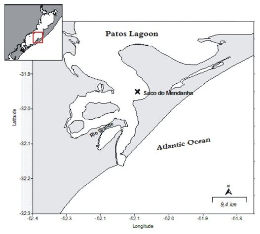
Figure 1. Location of the sediment collection point (Saco do Mendanha).

 

The sediments were collected with a gravity corer at a point [S 31°51.216, W 52°04.174] in the Saco do Mendanha, on board of the boat LARUS in April 2009. Four corers were collected in PVC tubes (ID 75 mm and 1 m length), that have been previously cleaned.

The corer uses the gravity force to penetrate the sediment allowing the collection of intact vertical profiles. After collecting the corers, they were sealed with PVC caps and placed in an upright position until the arrival at the laboratory. In the laboratory, two fractions of the core were removed, the first between 0 and -5 cm, and second between -15 and -20 cm, from the upper surface. All operation has been conducted in an inert hood (using nitrogen to purge the air from the hood), in such a way that the contact between the sample and atmospheric air was minimized, thus avoiding physico-chemical changes in the analyte.

 

Extraction of pore water

Each fraction of sediment samples was transferred to 500 mL HDPE bottles (Nalgene®), sealed and centrifuged for 30 min at 4000 rpm. After centrifugation, the supernatant (pore water) was transferred with a micropipette to a clean HDPE bottle. To analyze dissolved iron, an aliquot of the centrifuged pore water was filtered through a 0.2 μm cellulose acetate membrane in a Sartorius® system, acidified with HCl Suprapur MERCK® to pH 2.5 [10], ultraviolet (UV) irradiated for 6 hours, using a low pressure Hg vapor, and stored frozen until the analysis. For speciation analysis, an aliquot of the centrifuged pore water was taken and immediately filtered, as previously described, without the acid addition, and frozen until the analysis. All these steps were carried out in a closed hood with a continuous nitrogen flow to avoid the contact of the samples with atmospheric oxygen and the loss of analyte by oxidation and precipitation.

 

Experiments

The polyethylene bottles used to storage of samples, the voltammetric cell and general glassware used in the experiment were first washed with ultrapure water (resistivity 18.2 MΩ cm), and left in a 5 mol L^-1 HNO3 (Merck®) bath for five days. After this period the material was rinsed three times and kept immersed in ultra pure water for 24 hours. The filtration system is soaked in 1 mol L^-1 HCl (Merck®) for three days, and after washed with ultrapure water. The material was dried in laminar flow hood (Labconco®) and individually wrapped in PVC. The dissolved iron analysis occurred after the samples were UV irradiated to destroy the organic matter. A homemade UV irradiator was used, consisting of a mercury vapor lamp (125 W) and of 100 mL quartz tubes (with samples) disposed around the lamp. The internal temperature was kept below 70 °C by circulating air. The voltammetric analyses were performed in a EG&G PAR 384B potentiostat and a system of three electrodes EG&G PAR 303A, consisting in a working electrode of hanging mercury drop, platinum wire as auxiliary electrode and a reference electrode Ag/AgCl in 3 mol L^-1 KCl.

The buffer solution of 4-(2-hydroxyethyl)-piperazine-1-propane sulfonic acid (HEPPS, Fluka) 1 mol L^-1 was prepared in NaOH (0.5 mol L^-1), with final pH adjusted to 8.1. The signal was enhanced by using 0.4 mol L^-1 potassium bromate (KBrO3, J.T Baker); the 2,3-dihydroxynaphthalene (Fluka®) 0.020 mol L^-1 in methanol was the added ligand, to form an electroactive complex with iron. The sample deoxygenation was performed by purging with nitrogen analytical grade. This work was developed in different stages: (a) optimization of voltammetric parameters; (b) validation of the method; (c) collection of sediment samples; (d) extraction of pore water; and (e) application of the validated method in natural samples of pore water. The square wave cathodic stripping voltammetry (SWV) was chosen due to its sensitivity and analytical speed. The optimization of voltammetric parameters was performed for the DHN final concentration, frequency, deposition time, conditioning potential, scan rate and pulse height. Some instrumental parameters were pre-established, such as: initial potential (-0.4 V), final potential (-0.8 V), initial purge time (300 s), purge time between replicas (60 s), equilibrium time (10 s) and conditioning time (10s). The optimized values for the voltammetric determination of iron were: final DHN concentration 0.040 mol L-1, frequency 10 Hz, deposition time 0 s, conditioning potential -0.1 V, speed scanning 0.002 V s^-1 and pulse height 0.05 V. The figures of the merit evaluated were the linearity, the limit of detection (LOD), limit of quantification (LOQ), precision and accuracy.

Procedure for determination of dissolved and labile iron

The different species of iron were determined in samples of the overlying water, of the pore water in the first 5 cm depth of sediment and between -15 to -20 cm deep. To analyze the dissolved iron concentration, samples were diluted with ultrapure water. In the voltammetric cell were added 10 mL of diluted sample, 20 μL of 0.020 mol L^-1 DHN, 100 μL 1 mol L^-1 HEPPS and 500 μL of 0.4 mol L^-1 KBrO₃. Air was purged by nitrogen flow for 300 s. It was used the method of standard addition, with three additions of 20 μL iron standard solution 8.96×10^-6 mol L^-1. Current intensity was recorded in triplicate for each addition and the arithmetic mean was used to calculate the iron concentration. To ten voltammetric cells were added 10 mL of filtered pore water sample, an increasing iron concentration by standard additions (from 0 to 44.8×10-9 mol L^-1, final concentration), 20 μL of DHN (0.020 mol L^-1) and 100 μL of buffer HEPPS (1 mol L^-1). This batch of cells was kept overnight (ca. 17 hours) to the equilibrium to be established before analysis. The bromate was added to the cell just before the determination. The labile metal fraction was determined by CLEAdCSV. A titration curve was built plotting (total iron present in the sample) versus (current intensity), and its sensitivity (S) was used to calculate the labile iron (Equation 1), considering only the last points of the titration curve.

 

 

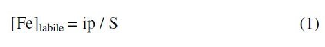
where ip is the current intensity at the first point of the titration curve - sample not fortified.

 

Results and discussion

Validation

The linearity was determined from successive additions of iron standard solution (8.96×10^-6 mol L^-1) to voltammetric cell. Fig. 2 shows the linearity up to 300×10^-9 mol L^-1, with a Pearson correlation better than 0.998.

 

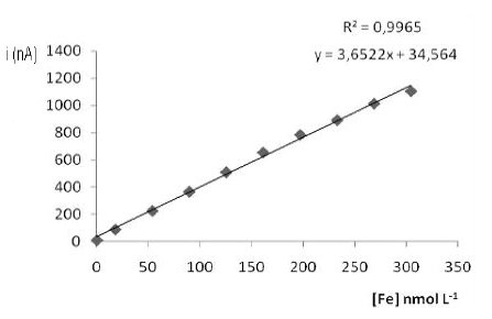
Figure 2. Analytical curve used to define the linearity to iron determination by adsorptive stripping voltammetry.

 

The detection and quantification limits, and the precision and accuracy of the method, were calculated using certified reference material (CRM) SLRS-4 (National Research Council Canada), which has 1.84×10^-6 mol L^-1 iron concentration. The calculation to determine the detection and quantification limits was performed using the standard deviation (3s) criterion for six replicates analysis of the CRM. The detection limit found was 0.30×10^-6 mol L^-1 and the quantification limit was 0.90×10^-6 mol L^-1. The precision was calculated based on the relative standard deviation (RSD) and was equal to 4.9%. The accuracy was determined from the recovery analysis of CRM samples and synthetic seawater fortified, being 98.28%.

The validated method was applied to analyze samples of pore water extracted from the sediment.

Fig. 3 shows analytical curves and voltammograms obtained in dissolved iron analyses to different depths.

 

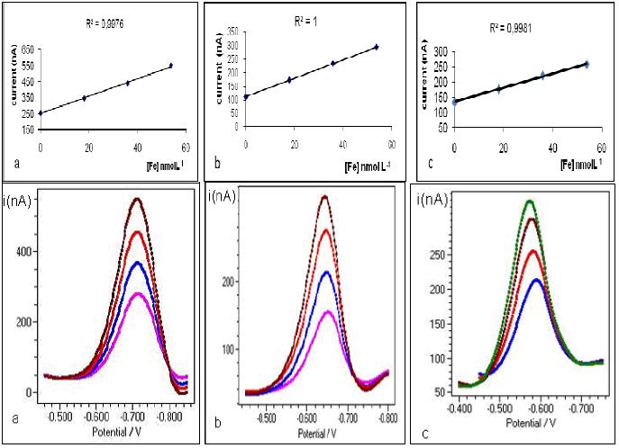
Figure 3. Analytical curves and voltammograms to dissolved iron. (a) overlaying water; (b) pore water from 0 to -5 cm; and (c) pore water from -15 to -20 cm depth.

 

All analytical curves had a Pearson's coefficient (r) better than 0.995, and the dissolved iron concentration in each fraction was determined, being showed in Table 1. Fig. 4 shows the titration and linearization curves used to analyze the chemical speciation of the iron in pore water (fraction between 0 and -5 cm). The linearization was done according to Van den Berg and Kramer (1984) [17], and the concentration of labile iron ([Fe]_labile, concentration of natural ligand (CL), and stability constant (K) were also calculated as proposed by those authors. The results for the chemical speciation of the iron are shown in Table 1.

 

Table 1. Results for overlaying water and pore water. Iron dissolved concentration ([Fe]_diss); iron labile concentration ([Fe]^labile); natural ligand concentration (CL); and stability constant (K).

 

 

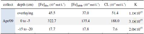
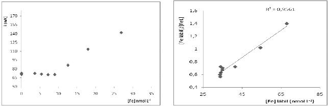
Figure 4. Titration curves in determining the concentration of iron in the labile fraction of 0 to -5 cm depth.

 

The upper fraction of sediment is characterized by intense biological activity and by remineralization processes. The anoxic, or suboxic, conditions prevailing in sediment, together with those processes previously listed, are the main responsible forces for the iron dissolved concentration. The bivalent iron, more soluble than the trivalent form, is stable in anoxic conditions, while the high concentration of natural ligands stabilizes the trivalent iron. Results in Table 1 show the dissolved iron and natural ligand (CL) concentration are effectively higher than in overlaying water or in pore water extracted from deeper layer.

The results of iron chemical speciation ([Fe]_labile; CL; K) are in consonance with dissolved iron results. The higher iron labile concentration occurs at the same time than higher CL and K, in other words, the presence of organic matter (high concentration of natural ligand) is important to stabilize iron, maintaining it in a labile form. However, the ratio [Fe]_labile/[Fe]_diss in the upper fraction (0 to -5 cm) is lower than the overlaying water (Table 1), what can be related with the nature of natural ligand in the system. If the complex has the same stability constant (K) in both fractions, the reason for the ratio [Fe]labile/[Fe]diss to be lower in the layer (0 to -5 cm) is because there are stronger natural ligands present there than in overlaying water, assuring iron to be soluble but not labile. As it is known, the concentration of the natural ligand and its stability constant is dependent on detection window used by CLE technique. It should be pointed out that the concentration of natural ligands measured (K ca 105) is proportionally lower in pore water (0 to -5cm) than in overlaying water. It is made clear comparing the ratio CL/[Fe]diss for the two fractions of water, 1.13 and 0.58 to overlaying and pore water, respectively.

 

Conclusions

The results pointed out that the proposed method exhibits excellent analytical conditions to determine the concentration of dissolved iron and its chemical speciation in sediment pore water. Although the method was originally developed to analyze iron in seawater, where levels are in the order of 10^-9 mol L^-1, the use of a proper dilution allows to use the method in matrix with the high concentrations of metal. The concentration of dissolved iron agrees with the values found by Belzile and colleagues [18] for the pore water, 0.35×10^-3 mol L^-1 between 0 and -5 cm depth and 50×10^-6 mol L^-1 in the interface water/sediment. It was stated the importance of the top layer in sediment, concerning the chemical speciation of iron. While in the stabilized sediment (deeper layer), as well as in overlaying water, high fraction of dissolved iron is present in labile form, in the top layer less than fifty percent of the dissolved iron is present as labile, probably because the natural ligands present are stronger than those present in overlaying water. The more stable iron complexes have an important function to transfer it from pore water to the water column.

 

References

1. J.A.B. Neto, M.W. Kersanach, S.M. Patchineelam, Poluição Marinha, Interciência-RJ. (2008) p. 197.         [ Links ]

2. J. Santos-Echeandia, R. Prego, A. Cobelo-Garcia, G. E. Millward, Marine Chem. (2009) 77.         [ Links ]

3. S. Emerson, R. Jahnke, D. Heggie, J. Marine Res. 42 (1984) 709.         [ Links ]

4. A. Widerlund, Marine Chem. 54 (1996) 41.         [ Links ]

5. P. Monterosso, P. Pato, M.E. Pereira, G.E. Millward, C. Vale, A. Duarte, Estuarine Coastal Shelf Sci. 71 (2007) 148.         [ Links ]

6. P.W. Boyd et al., Nature 407 (2000) 695.         [ Links ]

7. L.E. Brand, Limnol. Oceanogr. 48 (1991) 1756.         [ Links ]

8. P. Hyenstrand, E. Rydin, M. Gunnerhed, J. Plankton Res. 22 (2000) 1113.         [ Links ]

9. M. Gledhill, C.M.G. van den Berg, Marine Chem. 47 (1994) 41-54.         [ Links ]

10. C.M.G. van den Berg, H. Obata, Anal. Chem. 73 (2001) 2522.         [ Links ]

11. C.M.G. van den Berg, Analytical Chemistry 78 (2006) 156.         [ Links ]

12. A.L. Alvarado-Gámez, J. Campos-Fernández, Port. Electrochim. Acta 23 (2005) 209.         [ Links ]

13. T. Nagai, A. Imai, K. Matsushige, K. Yokoi, T. Fukushima, Limnology 5 (2004) 87.         [ Links ]

14. T. Nagai, A. Imai, K. Matsushige, K. Yokoi, T. Fukushima, Water Res. 11 (2007) 775.         [ Links ]

15. L.F.H. Niencheski, L.H. Windom, R. Smith, Mar. Pollut. Bull. 28 (1994) 96.         [ Links ]

16. L.F.H. Niencheski, L.H. Windom, R.G. França, J. Coastal Res. 39 (2006) 1040.         [ Links ]

17. C.M.G. van den Berg, J.R. Kramer, Marine Chem. 15 (1984) 1.         [ Links ]

18. N. Belzile, M. Filella, T. Deng, Y. Chen, Environ. Sci. Technol. 37 (2003) 1163.         [ Links ]

 

^*Corresponding author. E-mail address: setwotter@yahoo.com.br

 

Received 14 March 2010; accepted 12 May 2011