


 Inglês (pdf)
 Artigo em XML
 Referências do artigo
 Enviar este artigo por email
 Citado por SciELO
  Similares em
SciELO
Similares em
SciELO 
 Permalink
Introduction
The basic metals production is a minor economic activity in Costa Rica. The majority of these materials are obtained by importation. Therefore, it can be set as convenient for the country to know the corrosion mechanisms of basic metallic materials, in order to consider their effects on its economy. Corrosion losses are estimated to be about 3% of the country's gross domestic product (GDP). Much of this impact can be avoided with appropriate protective measures. The main losses in a tropical country are due to the atmospheric corrosion of structural materials, such as low CS or galvanized steel 1),( 2).
Costa Rica main urban areas are located away from the coast line, inside the geographic region known as WCV. WCV concentrates most of the country population (50%) and economic activities (60%). Hence, this sector is of great interest for the assessment of the basic metals deterioration 3-5.
WCV is considered an AB, surrounded by the volcanic mountain range to the north, and the foothills of the Talamanca mountain range to the south and the east. It has an average altitude of 1000 m above the sea level (m.a.s.l.), with elevations exceeding the 2500 m. The climate is monsoonal, with an average annual rainfall of 2300 mm/m-2, mainly between the months of May and November (rainy season). The temperature (T) ranges from 20 to 25 ºC, while the relative humidity (RH) varies from 70 to 90%, depending on the altitude and the time of the year. Winds have a main direction associated with the Alisios or Trade winds, in the NE towards the SW direction, according to the orography and seasonality 6-8.
In Costa Rica, atmospheric corrosion studies are generally associated to externally funded or company projects with specific purposes, both in terms of the selected location and the used materials. Some of them present only general information about WCV, for low steel alloys and galvanized Fe, without considering the climatic variability in that area 9),(10.
Atmospheric corrosion in WCV was proposed as a mild rural or light urban type of corrosion, with low levels of contamination, and mainly dependent on the meteorological parameters, especially RH, or its equivalent in terms of corrosion, and TOW. This is related to the C2 or C3 corrosion levels, as stated by ISO 9223 9-13. None of the studies mentioned any difference in the seasonality effect on corrosion. Meanwhile, Garita et al. (2014) performed a basic corrosion modeling estimate with atmospheric parameters, for WCV 14.
In this work, low CS corrosion was studied to evaluate if there was a seasonal effect, after the metal short exposure in WCV, and to examine different mathematical models for corrosion data estimation.
Methodology
The studied area is shown in Fig. 1. The study was conducted with low CS.
Low CS composition before analysis is detailed in Table 1, and compared with that stated by the American Society for Testing and Materials (ASTM) for A36 CS, which is commonly used as a standard 15-17.
CS composition was evaluated by optical emission spectrometry (OES), using a Leco model GDS500A spectrometer.
The low CS samples were cut into 100 mm x 50 mm x 1.5 mm coupons. They were initially cleaned with soap and water, to remove grease and dirt. Then, they were polished with wet sandpaper of increasing grades, up to 600 grit. Later, the specimens were cleaned in an ultrasonic bath, and rinsed with distilled water and acetone, before being dried in air. All the coupons were weighed and prepared for the exposure test 17-19.
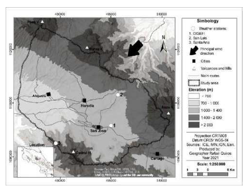
Table 1 Low CS composition and comparison with that stated by ASTM for A36 CS.
| Material | Fe% | C% | Mn% | Si% | S% | P% | Cu% |
| Exposed CS | 99.5 | 0.055 | 0.266 | 0.031 | 0.007 | 0.011 | 0.006 |
| ASTM - A36 CS | >99 | Max. 0.25 | - | Max. 0.4 | Max. 0.05 | Max. 0.04 | Min. 0.2 |
Corrosion monitoring stations were built based on ASTM G50-20 and G92-20 standards 17),(20. Their installation sites are shown in Table 2. These stations were located across WCV, in the main direction of the wind flow, from NE towards SW (see Fig. 1).
Table 2 Corrosion monitoring station installation sites.
| Site | North latitude | West longitude | Altitude (m.a.s.l.) |
| CIGEFI* | 09º 56' 11" | 84º 02' 43" | 1210 |
| San Luis | 10° 00' 54" | 84° 01' 36" | 1341 |
| Santa Ana | 09° 52' 54” | 84° 11' 14" | 1772 |
* Centro de Investigaciones Geofísicas (Research Center in Geophysics, University of Costa Rica).
For the corrosive atmospheric classification proposed by ISO 9223, climate parameters were evaluated based on meteorological data provided by the National Meteorological Institute (IMN) and the Costa Rican Institute of Electricity (ICE), at stations near the sampling sites. The considered parameters were T, RH, rainfall (R) and wind (W). TOW was estimated according to ISO 9223, by counting the number of hours when RH was greater than or equal to 80%, and T was higher than 0 ºC 13. Atmospheric pollutants were evaluated following ISO 9225 (2012), using humidity candles for chlorides (Cl), and passive monitoring, such as Passam AG (2012), for sulfur dioxide (SO2), ozone (O3) and nitrogen oxides (NOx) 21),(22.
Public volcanological data, on the dispersion of contaminants emitted by nearby volcanoes (Irazú, Turrialba, in the SE, and Poás, in the North of WCV), provided by the Volcanological and Seismological Observatory of Costa Rica (OVSICORI) and the Environmental Observatory of the National University, with the support of IMN and the Laboratory of Chemistry of the Atmosphere (LAQAT), were also analyzed. The influence of tropical storms was also considered 23.
CS samples corrosion assessment was performed through the weight loss (WL) gravimetric technique, by chemical pickling, according to ASTM G1 (2003), using the 3.35 method 18.
Two series of samples were exposed to the corrosion process in the rainy (from September 2018 to September 2019) and dry seasons (from March 2019 to April 2020), respectively.
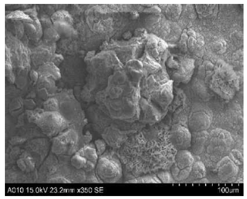
The 2, 6 and 12-month-old samples were additionally analyzed by Scanning Electronic Microscopy (SEM) and X-ray Diffraction (XRD). The SEM microscope was a Carl Zeiss Sigma 300 model, and the diffractometer was a Bruker XDS D8 Focus model.
Corrosion models
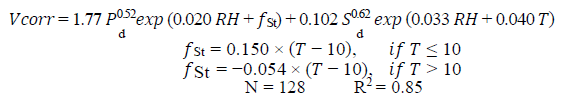
The annual values gravimetrically obtained were compared with those established by the model given in ISO 9223 13 for low CS, according to the climatic and pollution parameters for each site, as per the formula:
 ***
***
where Vcorr = corrosion rate in the first year (µm y-1), fst = factor for steel (due to the change of T effect on atmospheric corrosion from a critical temperature near to10 ºC), T = annual average temperature (°C), RH = annual average relative humidity, %Pd = annual average SO2 deposition (mg/m-2/d-1) and Sd = annual average Cl- deposition (mg/m-2/d-1).
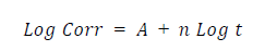
Some authors 14,24-26 proposed a corrosion model based on time, where the most simplified equation corresponds to:
 ***
***
where Corr = corrosion accumulated in time (µm), t = accumulated time (in years) and n = slope, which is inversely associated with the protection level of the oxide surface. The A constant is equivalent to Log (Corr), where Corr is the corrosion in the first year.
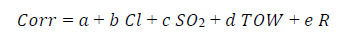
Other applicable models are lineal, logarithmic or bi-logarithmic 26-30 equations, which are stated as:
 ***
***
 ***
***
 ***
***
where TOW = accumulated time of wetness (in h), SO2 = accumulated SO2 deposition (mg/m-2), Cl = accumulated Cl- deposition (mg/m-2) and R = accumulated rain (mg/m-2). These equations were contrasted in different seasons, for each site, and by group.
Modeling control parameters
Three possible relationships between the experimental and modeling results were considered as control parameters: Pearson's correlation coefficient (PR2), which should be greater than 0.7, to be taken as acceptable; the residual sum of squares (RSS), a performance evaluator, which is expected to be minimum; and the Fisher's index (F) that should be higher than 100 31-33.
Prior to the iterative modeling process, Principal Component Analysis (PCA) and basic statistic tests (U Mann Whitney, Kruskal Wallis and Pearson's correlations factors) were initially carried out to determine the main factors 31),(32. Based on this, the models of the equations 3 and 4 were developed, considering that they must had more data than variables to be modeled.
Model fitting and parameter determination were performed in Python programming language, using the Pandas software library, for data management, and the stat models package, for parameters estimation and control parameters calculation.
Results and discussion
Corrosion and associated parameters
Corrosion assessment, at the sampling sites, and the meteorological and contamination data are shown in Tables 3 and 4, for rainy and dry seasons, respectively. All parameters are expressed in a cumulative form.
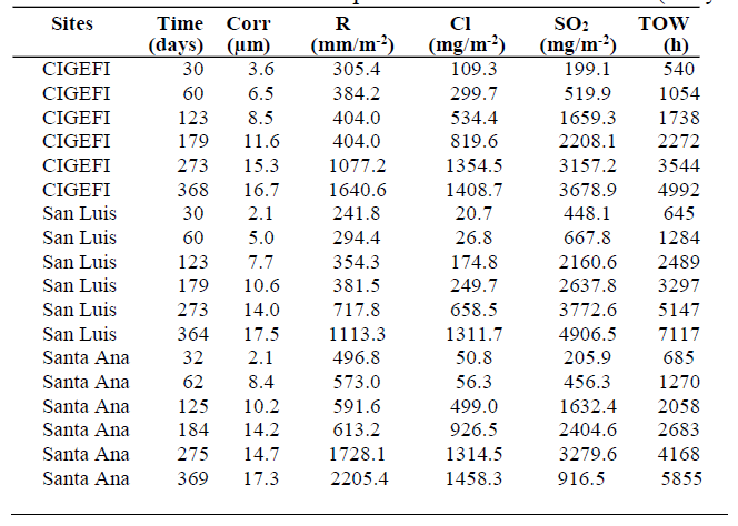
Table 4 Corrosion data and accumulated parameters for the second series (dry season).
| Sites | Time (days) | Corr (µm) | R (mm/m-2) | Cl (mg/m-2) | SO2 (mg/m-2) | TOW (h) |
| CIGEFI | 35 | 3.7 | 17.8 | 358.4 | 441.0 | 319 |
| CIGEFI | 64 | 6.1 | 244.8 | 418.5 | 853.1 | 769 |
| CIGEFI | 126 | 9.1 | 816.0 | 541.6 | 1081.7 | 1754 |
| CIGEFI | 189 | 12.2 | 1236.6 | 589.1 | 1470.8 | 2720 |
| CIGEFI | 274 | 14.1 | 1803.2 | 825.3 | 2748.3 | 4079 |
| CIGEFI | 399 | 17.9 | 1883.6 | 1083.7 | 3765.1 | 5328 |
| San Luis | 35 | 2.2 | 47.5 | 230.5 | 582.7 | 552 |
| San Luis | 64 | 4.4 | 190.5 | 344.9 | 1039.8 | 1145 |
| San Luis | 126 | 9.5 | 492.8 | 809.3 | 1480.7 | 2488 |
| San Luis | 185 | 11..8 | 728..7 | 1062.0. | 2268.7 | 3747 |
| San Luis | 274 | 15.1 | 1261.4 | 1611.9 | 3463.3 | 5686 |
| San Luis | 399 | 16.5 | 1402.1 | 1835.2 | 4630.0 | 8164 |
| Santa Ana | 32 | 2.8 | 226.5 | 363.5 | 299.6 | 338 |
| Santa Ana | 61 | 4.2 | 622.2 | 413.7 | 639.0 | 870 |
| Santa Ana | 123 | 8.4 | 1203.7 | 466.4 | 968.5 | 2034 |
| Santa Ana | 185 | 11.4 | 1592.2 | 563.0 | 1511.9 | 3172 |
| Santa Ana | 271 | 15..8 | 2402..0 | 867.6 | 2839.9 | 4830 |
| Santa Ana | 396 | 20.4 | 2505.9 | 1239.6 | 4413.7 | 6414 |
Note: The final time for the second series is longer than a year, because, on March 2020, the COVID19 pandemics caused mobilization restrictions in Costa Rica.
Table 5 shows the annual mean values of Cl, SO2, RH and T, while Table 6 presents the average W, NOx, and O3 data for the studied sites.
Table 5 Annual mean values of Cl, SO2, RH and T, for each season.
| Site | Cl (mg/m-2/day-1) | SO2 (mg/m-2/day-1) | RH (%) | T (ºC) | |||
| Rainy | Dry | Rainy | Dry | Rainy | Dry | Rainy Dry | |
| CIGEFI | 3.8 | 2.7 | 10.0 | 9.4 | 80.2 | 76.5 | 20.4 20.5 |
| San Luis | 3.6 | 4.6 | 13.5 | 11.6 | 87.5 | 90.1 | 17.8 18.2 |
| Santa Ana | 3.9 | 3.1 | 10.6 | 11.2 | 84.4 | 83.9 | 17.6 17.6 |
Table 6 Average annual W, NOx and O3 values at each site.
| Site | Wind direction | Wind speed (m/s-1) | O3 (µg/m-3) | NOx (µg/m-3) |
| Rainy Dry | Rainy Dry | Rainy Dry | ||
| CIGEFI | NE | 2.0 2.0 | 28.4 30.9 | 13.5 16.0 |
| San Luis | ENE | 3.0 3.0 | 27.2 30.8 | 7.1 7.7 |
| Santa Ana | N (*) | 3.0 3.1 | 33.2 41.7 | 4.6 5.8 |
Note: (*) The station has an orographic effect that causes the wind to move in a preferential N direction, instead of the usual NE route associated with the Alisios winds.
The average annual values for Cl and SO2 are low. These were defined, by ISO 9223, as S1 and P0, respectively. In a similar manner, the O3 and NOx values were found to be in the low contamination level, as stated by ISO 9223. All pollutant parameters measured for WCV indicate a rural or light urban atmosphere 13.
The analysis of the accumulated SO2 levels, as a function of time, shows a steady increase in them. The small differences between stations are associated to the volcanic activities wind dispersion effects. Regardless of that, the Cl levels are very dependent on the site and season of the year, and influenced by the seasonal wind speed.
The principal wind direction is the expected, and mostly affected by the strength of the Alisios wind (from the NE) in each season, and by orographic effects that produce a small increase in O3 in the Santa Ana site 34.
The mean RH value is relatively high, and usually above 80%, while T is above 17 ºC, being both relatively independent of the seasons. The accumulated R decreases from NE to SW, in WCV, almost equally in both seasons, with lower values than the historical mean in the San Luis and CIGEFI sites 6),(8.
The annual TOW values are mainly in the range of 5, with more than 5000 h, a considerably high figure 13),(35. The Corr values measured in both campaigns (started in the rainy or dry seasons) correspond to the C2 category in ISO 9223 13, in the range from 15 to 18 µm per year. This result is consistent with the concept of rural or light urban atmosphere and high TOW values 9),(14),(36),(37.
Volcanic activity and tropical storms
The volcanic activity during the studied period was low, mainly originated in the Turrialba volcano, as a result of eruptive emissions between September and December 2018, and in April 2019. The general SW wind direction (Alisios winds) transports most of the Turrialba emissions far from WCV, located to the NW. Part of these emissions were directed to WCV, in November and December, due to prevalent winds, but did not have a significant influence on the overall values. There were also slight emissions from the Poás volcano, between November and December 2018, but the main direction was towards other areas located in the WCV west side 23.
No tropical storms have affected WCV during the course of this work 38),(39.
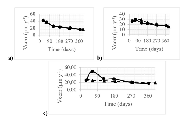
Figure 2 Vcorr values in both seasons (rainy: circles with full line; and dry: triangles with dashed line), in the stations of: a) Santa Ana, b) CIGEFI and c) San Luis, respectively.
Relationship between seasons
In all sites, accumulated Corr general trend was found to be logarithmic, while Vcorr had an exponential decay, which can be seen in Fig. 2, for all sites. Corr was dependent on the site characteristics, but not on the onset season, while Vcorr was affected by the onset season in the first months of corrosion.
The relation of Corr with each season is relatively linear, according to the equation which states that Corr (dry) = a Corr (rainy) + b, where the slope is near to 1 (see Table 7).
Table 7 Linear fit for the correlation between Corr dry vs. Corr rainy.
| Sites | a | b | R2 |
| Santa Ana | 1.0162 | 0.0124 | 0.9751 |
| CIGEFI | 0.9833 | 0.5789 | 0.9633 |
| San Luis | 1.1374 | -2.1735 | 0.8470 |
Vcorr values do not present peaks in the first months, for the Santa Ana site, while, on the other sites, this situation is observed, especially in the rainy season. The initial Vcorr values in the rainy season increase when the wind is moving from SW to NE, in WCV (see Fig. 2). CIGEFI and San Luis sites are clearly affected by R and RE effects, possibly because the decrease in the intensity of the Alisios winds brings moisture from the Pacific coast that concentrates in the WCV center and north side, due to the higher altitude of the volcanic mountain range 6-8.
SEM and DRX
The basic oxide composition is associated to goethite (G) and lepidocrocite (L), in proportions of 35 and 65%, respectively, for the one-year analysis. The values at 2 and 6 months show a similar composition and proportion, with a little trend towards a decrease in L values and an increase in G values, with time. This process is related to the oxide surface stabilization.
Data models
The values obtained for the different models, considering the climatic season and sampling sites, are presented below.
ISO model (equation 1) and measured values
The equation 1 values from ISO 9223 always present higher results than the measured values obtained for WCV (Table 8). This is consistent with the tropical conditions and low contamination levels in WCV. In this situation, the equation is not so representative, because it is mostly originated from subtropical data that reflect different climacteric conditions 9),(14,28,36,37,40,41.
Table 8 Annual Vcorr values (µm/y-1) from ISO 9223 (eq. 1), and those measured in each site.
| A (m.a.s.l.) | Site | ISO 9223 | Measured values | |||
| Rainy | Dry | Rainy | Dry | |||
| 1210 | CIGEFI | 24.1 | 20.3 | 16.7 | 17.9 | |
| 1341 | San Luis | 34.1 | 35.3 | 17.5 | 16.5 | |
| 1717 | Santa Ana | 29.5 | 28.7 | 17.3 | 20.4 | |
Note: actual dry season values were calculated for the sampling time.
Corr vs. time model (equation 2)
Table 9 shows the correlations associated with equation 2, for the stations, in the different seasons, where Log (Corr) is the experimental value related to A, obtained at each site.
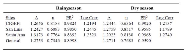
The sites show correlations with PR2 values generally higher than 0.9, regardless of the season. Parameter A has, in general, a good correspondence with Log (Corr) of real values in one year, and it is similar in all equations.
The n constant has values in the range from 0.60 to 0.85, with an average of 0.73 to 0.76, for the general equations. These values imply corrosion moderate or partial attenuation by the oxides surface formation, which tends to stabilize Vcorr over time, in areas such as WCV (14, 26).
While the general equations by season are similar, they provide a general way for estimating low CS corrosion over time, for WCV. In these equations, the correlation in the dry season is more stable in the early stages, and less dependent on the conditions of each site, thus presenting a better PR2. The global equation based in equation 2, for WCV, is:
 ***
***
Equation 2 usually provides a good fit for low CS in less contaminated media, over short to medium time periods (1 to 5 years) 9,14,24-30,42-46.
Lineal and logarithmic models (equations 3 and 4)
Pearson’s correlation coefficients for each parameter, in relation to corrosion, were calculated (p > 0.01). The values, for all parameters, have a good correlation (more than 0.7). SO2 and TOW have the best correlations, followed by Cl and R (see Table 10).
Table 10 Pearson's correlation coefficient between variables.
| Corr (µm) | R (mm/m-2) | Cl (mg/m-2) | TOW (h) | SO2 (mg/m-2) | |
| Corr | 1 | 0.788 | 0.827 | 0.949 | 0.903 |
| Rain | 1 | 0.671 | 0.765 | 0.771 | |
| Cl | 1 | 0.853 | 0.842 | ||
| TOW | 1 | 0.952 | |||
| SO2 | 1 |
Comparisons between seasons (U Mann Witney, p > 0.05) and sites (Kruskal Wallis, p > 0.05) show no significant differences.
Since there are no significant seasonal differences, the modeling was globally considered by site, and in WCV, with different numbers of variables. As stated in the methodology, the control parameters to evaluate the quality of models were PR2, RSS and F.
The best results for equation 3, in its lineal and logarithmic forms, were:
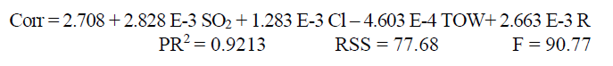 ***
***
 ***
***
There was no substantial improvement when using the linear form. Similar equations were obtained for tropical environments, by other authors (10, 14, 26-30, 36, 37, 40, 41, 43-46).
The most basic equations with one parameter are the ones that include TOW, expressed as a logarithmic regression. TOW is usually the most important parameter to control the corrosion processes in tropical environments, especially far from the coast, and with low levels of pollutants 9,11,14,26,35-37,41-46.
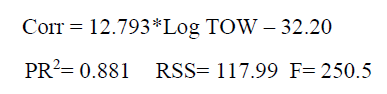 ***
***
Table 11 presents equation 4 coefficients for the best correlations with a different number of global variables, in the whole WCV.
Equation 4 is an extension of equation 2. The high correlation of corrosion with time limits the improvement obtained with the addition of new variables. This is seen in a somewhat higher PR2 value, with respect to equation 5, even when there is a decrease in the number of variables (Table 11) 14,43.
The most influential variable on corrosion, in equation 4, over time, is SO2. Even so, equation 4 does not improve corrosion estimation, being more complex than equations 2 and 3.
Table 11 Best correlation obtained for WCV, in general, for equation 4.
| # variables | Log t | Cl | SO2 | TOW | R | PR2 | RSS | F | |
| a | n | b | c | d | e | ||||
| 5 | 1.5435 | 1.0130 | 6.99E-06 | -6.89E-05 | 3.28E-06 | -3.17E-05 | 0.9427 | 1.71E-01 | 98.80 |
| 4 | 1.5421 | 1.0119 | -6.48E-05 | 8.00E-06 | ND | -2.99E-05 | 0.9427 | 1.71E-01 | 127.54 |
| 3 | 1.5442 | 1.0136 | ND | -6.31E-05 | ND | -2.93E-05 | 0.9427 | 1.71E-01 | 175.40 |
| 2 | 1.4926 | 0.9650 | ND | -6.13E-05 | ND | ND | 0.9408 | 1.76E-01 | 262.19 |
Early mathematical models of atmospheric corrosion were based on equations 2 and 3. These were used both cumulatively, and for sites comparison on annual corrosion 9,11,14,24-29,46-49. From these models, the main parameters to be considered for atmospheric corrosion, according to the environment, were established. For the case of rural or light urban atmospheres, the environmental factors were more important than the pollutants, obtaining better relationships with time and TOW. Subsequent studies in rural tropical bionetworks showed the strong influence of environmental factors, with higher corrosion rates than those of other subtropical-ecosystems under the same ecological conditions 9,10,14,24,36,37,40,43,45,46,48,50-56.
For WCV, equation 2 is presented as a model with a very good correlation between Corr and time, according to equation 5, while equation 3 generates a complex model of which simplification in rural tropical environments tends to be a function of t, RH and/or TOW 14,28,36,37,43,45,50-54. This agrees, in this case, with the result proposed for WCV, in equation 8.
Equation 4 arises within the process of improving corrosion modeling, by proposing a combination between equations 2 and 3. This equation improves the results, when the contamination effect is more important than time dependence. For WCV, there was no substantial improvement in the corrosion evaluation, and the dependence was associated with time and SO214,26-30,33,50,55,56.
In a similar way, equation 1, stated in ISO 9223, arises from worldwide corrosion evaluations. In this one, there are few tropical data within rural environments, so, it usually gives overestimated values, as in the WCV case 14,27,28,41,46,48,52,55,56.
Tropical corrosion assessments in rural environments do not show significant differences in relation to seasonality. However, they do show initial corrosion rates dependent on the onset corrosion time, and in relation to TOW levels 37,50,51. This is consistent with the results obtained for WCV.
Conclusions
The final low CS Corr values, after one year of exposure, did not show significant differences with the starting climatic season, or with the monitoring site at WCV. On the other hand, the initial corrosion values, during the first six months, were dependent on the site climatic conditions. Vcorr values were higher when atmospheric corrosion started during the rainy season and the sites had less rainfall, although there were high TOW values. Because of the above, the modeling was reduced to a single environment independent of the climatic season. While low pollution decreases the influence of these parameters on complex models, making simplified models using time or TOW produces adequate and less complex results. The ISO 9223 equation estimation for annual corrosion is very high, possibly because it is based on measurements in nontropical environments.
Acknowledgements
Special thanks to the National Meteorological Institute and the Costa Rican Electricity Institute, for providing the WCV meteorological data. The actual corrosion data were obtained from the measurement of the sites located at the facilities of the National Power and Light Company and the Ministry of Security. This study was funded by the National Council of University Presidents (CONARE) of Costa Rica, as part of a collaborative project among the State Distance University (UNED-VINVES-6-1050), the University of Costa Rica (UCR-VI-805-B8-650), the National High Technology Center (CeNAT-VI-269-2017), the National University (UNA- SIA: 0600-17) and the Costa Rica Institute of Technology (ITCR-VIE 1490-021).
Rodríguez-Yáñez acknowledges the support of the Innovation and Human Capital for Competitiveness Program (PINN) of the Ministry of Science, Technology and Telecommunications (MICITT) of Costa Rica.

